Mortality Risk Management

(1)

5-8-2006

Mortality Risk Management

Yijia Lin

Follow this and additional works at:https://scholarworks.gsu.edu/rmi_diss

This Dissertation is brought to you for free and open access by the Department of Risk Management and Insurance at ScholarWorks @ Georgia State University. It has been accepted for inclusion in Risk Management and Insurance Dissertations by an authorized administrator of ScholarWorks @ Georgia State University. For more information, please [email protected].

Recommended Citation

Lin, Yijia, "Mortality Risk Management." Dissertation, Georgia State University, 2006. https://scholarworks.gsu.edu/rmi_diss/14

(2)

In presenting this dissertation as a partial fulfillment of the requirements for an advanced degree from Georgia State University, I agree that the Library of the University shall make it available for inspection and circulation in accordance with its regulations governing materials of this type. I agree that permission to quote from, or to publish this dissertation may be granted by the author or, in his/her absence, the professor under whose direction it was written or, in his absence, by the Dean of the Robinson College of Business. Such quoting, copying, or publishing must be solely for scholarly purposes and does not involve potential financial gain. It is understood that any copying from or publication of this dissertation which involves potential gain will not be allowed without written permission of the author.

(3)

All dissertations deposited in the Georgia State University Library must be used only in accordance with the stipulations prescribed by the author in the preceding statement.

The author of this dissertation is: Yijia Lin

The director of this dissertation is: Samuel H. Cox

Department of Risk Management and Insurance Georgia State University

(4)

BY

Yijia Lin

A Dissertation Submitted in Partial Fulfillment of the Requirements for the Degree Of

Doctor of Philosophy

In the Robinson College of Business Of

Georgia State University

GEORGIA STATE UNIVERSITY ROBINSON COLLEGE OF BUSINESS

(5)

(6)

This dissertation was prepared under the direction of Yijia Lin’s Dissertation Committee. It has been approved and accepted by all members of that committee, and it has been accepted in partial fulfillment of the requirements for the degree of Doctor of Philosophy in the Robinson College of Business of Georgia State University.

H. Fenwick Huss, Dean

DISSERTATION COMMITTEE Samuel H. Cox Chair Andrew Cairns Martin F. Grace Harold D. Skipper Shaun Wang

(7)

BY Yijia Lin

2006 Committee Chair: Samuel H. Cox

Major Academic Unit: Department of Risk Management and Insurance

This is a multi–essay dissertation in the area of mortality risk management. The first es-say investigates natural hedging between life insurance and annuities and then proposes a mortality swap between a life insurer and an annuity insurer. Compared with reinsurance, capital markets have a greater capacity to absorb insurance shocks, and they may offer more flexibility to meet insurers’ needs. Therefore, my second essay studies securitization of mor-tality risks in life annuities. Specifically I design a mormor-tality bond to transfer longevity risks inherent in annuities or pension plans to financial markets. By explicitly taking into ac-count the jumps in mortality stochastic processes, my third essay fills a gap in the mortality securitization modeling literature by pricing mortality securities in an incomplete market framework. Using the Survey of Consumer Finances, my fourth essay creates a new finan-cial vulnerability index to examine a household’s life cycle demand for different types of life insurance.

(8)

Acknowledgments

It has been a great pleasure working with the faculty, staff, and students at Georgia State University, during my tenure as a doctoral student. This work would never have been possible if it were not for the freedom I was given to pursue my own research interests, thanks in large part to the kindness and considerable mentoring provided by Samuel Cox, my long-time advisor and committee chair. The members of my dissertation committee were truly remarkable. As the “outside” member of my committee, Andrew Cairns brought a much-needed scientific perspective to my work, editing skills, and a common sense view that improved the final product. It was Martin Grace’s guidance and seminar on insurance economics in 2002 that convinced me to think of my own research and finished one of essays in my dissertation. Harold Skipper also deserves a great deal of thanks, for it was his class on life insurance in 2002 that introduced me to the life insurance industry and provided the foundation to the work described in this dissertation. I also thank Shaun Wang who was always willing to answer questions, and remained a strong source of support throughout the course of my research.

I have benefited greatly from the generosity and support of many faculty members. In particular, I would like to thank Richard Phillips for his encouragement and willingness to go the extra mile to help a student. Special thanks also go to Sanjay Srivastava for boundless kindness and enthusiasm in his roles — teacher and chairperson. I would like to thank William Feldhaus for good advise and always being complementary. I am very grateful to Lorilee Schneider for giving me good teaching advise.

My study at Georgia State University has benefited from the administrative help of many people. Libby Crawley and Shannon Mosher provided me with exceptional administrative help. Mike Cohen always helped me in any way. I would also like to thank Jean Miller for

(9)

there are three people that made the completion of this dissertation possible by guiding me through various stages of my education. Early in life, as a primary school student, I crossed paths with Yuanfen Lin. This woman encouraged me and made me hungry for knowledge. Mr.Wei Tan is a talented teacher, wise and caring advisor. I will never pass a milestone in my life without remembering that it was he who convinced me failure once did not mean the end of the world. While an undergraduate in insurance and a master student in finance and insurance both in the Beijing Technology and Business University, I met Professor Xujin Wang. I am forever indebted to him not only for the way he led me to insurance field, but also for the myriad ways he supported me in all of my goals.

I also thank my parents for always being there when I needed them most, and for sup-porting me through all these years. Finally, this dissertation is dedicated to my greatest blessing, my husband, the most decent and loving person I have ever known. Going through difficulties hand by hand with him gives me magic strength and courage. Thank him for all his unconditional love and understanding. A lifetime with him will always be too short.

(10)

List of Tables

2.1 Summary Statistics from 1995 to 1998 . . . 14

2.2 Relationship between Annuity Price and Natural Hedging . . . 16

3.1 Market Price of Risk based on the One-Factor Wang Transform . . . 39

3.2 Improvement Levels for Three Age Groups . . . 39

3.3 Mortality Bond Price and Reinsurance Premium . . . 43

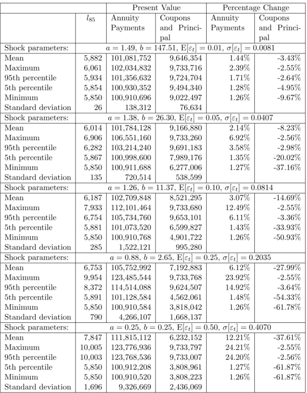
3.4 Simulation Results Based on Different Mortality Shock Assumptions . . . 48

3.5 Effect of Expense Rate on Prices . . . 49

3.6 December 2004 Earthquake and Tsunami Death Toll and Percentage Excess Death Rates by Country . . . 54

3.7 Regression Estimates of Mortality Projection Model . . . 59

4.1 Property and Life Insurance Securitization Issuance . . . 66

4.2 Market Price of Risk based on the Two-Factor Wang Transform . . . 71

4.3 Maximum Likelihood Estimates . . . 77

5.1 Summary Statistics for the Survey of Consumer Finances 1992, 1995, 1998 and 2001 Waves . . . 105

5.2 Life Cycle Relationship: Net Amount at Risk and Financial Vulnerability Index109 5.3 Life Cycle Relationship: Term Life Insurance and Financial Vulnerability Index110 5.4 Life Cycle Relationship: Sum of Net Amount at Risk and Term Life Insurance and Financial Vulnerability Index . . . 111

5.5 Life Cycle Relationship: Life Insurance and Household’s Portfolio in 2001 . 115 5.5 Life Cycle Relationship: Life Insurance and Household’s Portfolio in 2001 (Continued) . . . 116

5.5 Life Cycle Relationship: Life Insurance and Household’s Portfolio in 2001 (Continued) . . . 117

5.5 Life Cycle Relationship: Life Insurance and Household’s Portfolio in 2001 (Continued) . . . 118

5.6 Estimation Results of the Heckman Model . . . 121

(15)

5.8 Life Cycle Relationship: Life Insurance and Household’s Portfolio with Im-puted Housework Value in 2001 . . . 124 5.8 Life Cycle Relationship: Life Insurance and Household’s Portfolio with

Im-puted Housework Value in 2001 (Continued) . . . 125 5.8 Life Cycle Relationship: Life Insurance and Household’s Portfolio with

Im-puted Housework Value in 2001 (Continued) . . . 126 5.8 Life Cycle Relationship: Life Insurance and Household’s Portfolio with

(16)

1

Introduction and Overview

Mortality risk management is the process of identifying mortality risk exposures faced by an insurance company, a pension plan or an individual and selecting the most appropriate techniques for treating them (Rejda, 2005). Mortality risk management is critical to the financial stability of an insurance company, a pension plan or a household. My dissertation is a four–essay dissertation. It proposes new techniques for insurers and pension plans to manage mortality risk and examines households’ life insurance demand.

Froot and Stein (1998) develop a framework for analyzing the capital allocation and capital structure decisions facing financial institutions. Their model suggests that the hurdle rate of an investment opportunity consists of two parts: the standard market-risk factor and a factor for unhedgeable risk. Until now, little attention has been paid to the risk premium of unhedgeable mortality risks. In the first essay, I find evidence that annuity writing insurers who naturally hedge their annuity risk by also writing life insurance are able to charge lower premiums than do otherwise similar insurers. The evidence suggests that insurers who utilize natural hedging, a form of business diversification, have a competitive advantage.

(17)

Moreover, the insurer may prefer business focus rather than diversification, as expanding the number of activities of the firm is not without costs (Denis et al., 1997; Comment and Jarrell, 1995; Berger and Ofek, 1995; Lamont and Polk, 2002; Servaes, 1996; Scharfstein and Stein, 2000). Thus, I design a set of securities that I call mortality swaps and demonstrate that insurers can use the swaps to achieve the benefit of natural hedging without actually “diversifying” the business of the insurers.

An important recent innovation in financial markets is the securitization of mortality risks for catastrophic events such as natural disasters or exceptional improvements in life ex-pectancy. Mortality securitization has the potential to enhance the capacity of the insurance industry and allow it to efficiently spread risks beyond life insurance markets. Moreover, it provides an additional way to diversify an investor’s portfolio as mortality risk may be uncorrelated to or have low correlation with any other financial risk that underlies stock or bond price movements. The purpose of my second essay is to explain the rationale for the existence of mortality-based securities and to develop an equilibrium model that can be used to price the proposed mortality securities. I focus on individual annuity data, although the modeling techniques could be applied to other lines of annuity or life insurance.

The securitization of mortality risks is gaining more attention from investors. The first two publicly known mortality securities are the Swiss Re mortality bond and the European Investment Bank (EIB) longevity bond. Morgan Stanley reports that investors’ appetite for the Swiss Re bonds was strong while, on the other hand, the EIB bond has not sold well. The purpose of my third essay is to explain the interesting yet opposite market outcomes for these two securities.

I begin by developing a mortality stochastic model that allows for jump risk. I then consider the problem of pricing contingent claims on mortality bonds in an incomplete market framework. My results suggest that the Swiss Re bonds compensated investors with a risk premium that was approximately 90 percent higher than our model. On the other hand, the model suggests the EIB bonds charged UK pension plans a higher risk premium than did the insurance market for a similar level of longevity risk. Thus, the model explains why investors had a strong appetite for the Swiss Re bonds and not the EIB bonds. The research should also enable investors of future mortality bonds to understand better the uncertainty and pricing associated with catastrophic mortality risk securities.

Using the Survey of Consumer Finances my fourth essay examines a life cycle demand model for different types of life insurance. Specifically, I test for consumers’ avoidance of income volatility as a result of the death of a wage-earning household member through the

(18)

purchases of life insurance. The primary innovation in this research is that I develop a financial vulnerability index to control for the risk to a household and show, in contrast to previous research that there is a positive relationship between financial vulnerability and the amount of term life or total life insurance purchases. In addition, I find older consumers use less life insurance to protect a certain level of financial vulnerability than do younger consumers. My results are robust no matter whether or not I take into account non-monetary contribution of family members by imputing their housework value.

In summary, my dissertation examines mortality risk management for insurers, pension plans and individuals. My first essay investigates natural hedging and proposes and prices a mortality swap between a life insurer and an annuity insurer. My proposed mortality swaps may help stabilize the cash outflows of life insurers and annuity insurers. Compared with insurance markets, financial markets have much greater capacity to absorb catastrophe risks. My second essay suggests that life insurer may transfer mortality risks to capital markets via a mortality bond to increase their underwriting capacity. If so, life insurers are able to share the “bigger cake” of annuity markets if the U.S. reforms its social security system. Mortality securitization modeling is still an open question in the asset pricing literature. My third essay proposes a model to price mortality securities in an incomplete market framework with jump processes. This model nicely explains the opposite market outcomes of the first two mortality bonds. Similar to insurance companies, households also need to manage their mortality risks that arise from the death of wage-earning members. My fourth essay proposes a new financial vulnerability index to explore whether there is a life cycle relation between a household’s financial vulnerability and its life insurance holdings. The Overall, my dissertation will fill several gaps in the literature on mortality risk management.

(19)

2

Natural Hedging of Life and Annuity

Mortality Risks

The values of life insurance and annuity liabilities move in opposite directions in response to a change in the underlying mortality. Natural hedging utilizes this to stabilize aggregate liability cash flows. I find empirical evidence that suggests that annuity writing insurers that use natural hedging also charge lower premiums than otherwise similar insurers. This indicates that insurers that are able to utilize natural hedging have a competitive advantage. In addition, I show how a mortality swap might be used to provide the benefits of natural hedging.

2.1 Introduction

If future mortality improves relative to current expectations, life insurer liabilities decrease because death benefit payments will be later than expected. However, annuity writers have a loss relative to current expectations because they have to pay annuity benefits longer than expected. If mortality experience deteriorates, the situation is reversed: life insurers have losses and annuity writers have gains. Natural hedging utilizes this interaction of life insurance and annuities to a change in mortality to hedge against unexpected changes in

(20)

future benefit payments.

The purpose of this paper is to study natural hedging of mortality risks and to propose mortality swaps as a risk management tool. Few researchers investigate the issue of natural hedging. Most of the prior research explores the impact of mortality changes on life insurance and annuities separately, or investigates a simple combination of life and pure endowment life contracts (Frees et al., 1996; Marceau and Gaillardetz, 1999; Milevsky and Promislow, 2001; Cairns et al., 2006). Studies on the impact of mortality changes on life insurance focus on “bad” shocks while those on annuities focus on “good” shocks.

Wang et al. (2003) analyze the impact of the changes of mortality factors and propose an immunization model to hedge risks based on mortality experience in Taiwan. Life insurance and annuity mortality experience can be very different, so there is “basis risk” involved in using annuities to hedge life insurance mortality risk. Their model cannot pick up this basis risk.

Marceau and Gaillardetz (1999) examine the calculation of the reserves in a stochastic mortality and interest rates environment for a general portfolio of life insurance policies. In their numerical examples, they use portfolios of term life insurance contracts and pure endowment polices, like Milevsky and Promislow (2001). They focus on convergence of simulation results. There is a hedging effect in their results, but they do not pursue the issue.

This paper proceeds as follows: In Section 2.2, I use an example to illustrate the idea of natural hedging. In Section 2.3, using market quotes of single–premium immediate annuities (SPIA) from A. M. Best, I find empirical support for natural hedging. That is, insurers that naturally hedge mortality risks have a competitive advantages over otherwise similar insurers. In Section 2.4, I propose and price a mortality swap between life insurers and annuity insurers. Section 2.5 is the conclusion and summary.

2.2 Example

This example illustrates the idea of a natural hedge. Consider a portfolio of life contingent liabilities consisting of whole life insurance policies written on lives age 35 and immediate life annuities written on lives age 65. If mortality improves, what happens to the insurer’s total liability? We know that on average, the insurer will have a loss on the annuity business and a gain on the life insurance business. If mortality declines, the effects are interchanged. This example shows what can happen if mortality risk increases as a result of a common shock. Here are my assumptions:

(21)

2. The annuity has an annual benefit of 510 and it is issued as an immediate annuity at age 65.

3. The face amount of life insurance on age 35 is 100,000 and the life insurance is issued at age 35. For this amount of insurance, the present value of liabilities under the life insurance and under the annuity are about equal.

4. Life insurance premiums and annuity benefits are paid annually. Death benefits are paid at the end of the year of death.

5. The initial number of lives insured,`35, is 10,000 which is the same as that of annuitants

`65.

6. The mortality shock is expressed as a percentage of the force of mortalityµx+t, so it

ranges from -1 to 1, that is, −1 ≤ ≤ 1 with probability 1. Without the shock, the survival probability for a life age x at year t is px+t = exp(−µx+t). With the shock,

the new survival probabilityp0_x₊_t can be expressed as:

p0_x₊_t= (e−µx+t₎1− _{= (}_p

x+t)1−.

If 0 < ≤ 1, mortality experience improves. If −1 ≤ < 0, mortality experience deteriorates.

7. The term structure of interest rates is flat; there is a single interest rate, i= 0.06.

2.2.1 Life Insurance

For the life insurance, the present value of 1 paid at the end of the year of death isvk+1 _and

the expected present value is

Ax = ∞ X

k=0

vk+1kpxqx+k

where x is the age when the policy issued (x = 35 in this example). For a benefit of f the expected present value is f Ax.

The present value of 1 per year, paid at the beginning of the year until the year of death, is

¨

a_K₍_x_{) + 1} = 1−v

K(x)+1

(22)

The expected present value ¨ ax= E h ¨ a_K₍_x_{) + 1}i= ∞ X k=0 vkkpx.

The net annual premium rate for 1 unit of benefit is determined so that the present value of net premiums is equal to the present value of benefits. This means

Px¨ax =Ax

and for a benefit of f the annual premium is

f Px =f Ax/¨ax.

If the insured dies at K(x) = t, then the insurer’s net loss is the present value of the payment, less the present value premiums. For a unit benefit, the loss is

L=vK(x)+1−Pxa¨_K₍_x_{) + 1} =vK(x)+1−Px

1−vK(x)+1

d .

It follows from the definition of the net premium Px that the expected loss is zero. For

a benefit of f, the loss is f L. Of course, the loss can be negative in which case the result turned out in the insurer’s favor. On average, the loss is zero.

2.2.2 Annuities

For an annuitant age y, the present value of 1 per year paid at the beginning of the year is ¨

a_K₍_y_{) + 1} = 1−v

K(y)+1

d .

The expected present value

¨ ay = E h ¨ a_K₍_y_{) + 1}i = ∞ X k=0 vkkpy.

The policy is purchased with a single payment of ¨ay. In my exampley= 65 and the mortality

table is based on annuity experience. For an annual benefit of b, the net single premium is

ba¨y. The company’s loss per unit of benefit is

¨

(23)

2.2.3 Portfolio

The portfolio has a life insurance liability to pay a benefit of f at the end of the year of the death and a liability to pay a benefit of b at the beginning of each year as long as the annuitant is alive. The total liability is

f vK(x)+1+ba¨_K₍_y_{) + 1}.

To offset the liability the company has

f Px¨a_K₍_x_{) + 1} +b¨ay.

The difference is the total loss:

L=f vK(x)+1+bä_K₍_y_{) + 1} −f Pxä_K₍_x_{) + 1} −bäy.

The expected loss is zero. However, this expectation is calculated under the assumption that the mortality follows the tables assumed in setting the premiums. If we replace the before–shock lifetimes with the after shock lifetimes, what happens to the loss?

2.2.4 Results

Figure 2.1 shows the percentage deviation of the present value of benefits from the life insurance premiums and that of annuity payments from the total annuity premium collected at time t = 0. I also show the percentage of deviation from the present value of total premiums collected. Each result includes a shock improvement or deterioration relative to the table mortality, modelled by multiplying the force of mortality by a factor 1− in each year. With a small mortality improvement shock = 0.10, annuity insurers will lose 2.0 percent of their expected total payments. In this scenario, life insurers will gain 5.0 percent of their expected total payments. If the above life insurance and annuity are written by the same insurer, the shock has a much smaller effect on its business (a 1.5 percent gain). With a small mortality bad shock =−0.10, annuity insurers will gain 1.9 percent of their expected total payments. In this scenario, life insurers will lose 4.8 percent of their expected total payments. If the above life insurance and annuity are sold by the same insurer, a bad shock has little effect on its business (a 1.4 percent loss). When there is a big good shock

(24)

-0.4 -0.2 0.2 0.4 -20 -10 10 20 Life Annuity Total

Figure 2.1: The percentage deviation of the present value of benefits from the life insurance premiums, that of annuity payments from the total annuity premium collected and that of total premiums collected at time t = 0. The y–axis represents the percentage loss and the

x–axis represents different levels of shock improvement or deterioration factor .

life insurer will gain 28.0 percent of their total expected payments on average. The overall effects will be 7.9 percent gain on a big good shock. Writing both life and annuity business reduces the impact of a big bad shock = −0.50 to a 7.0 percent loss. I have illustrated the idea of natural hedging and I conclude that writing both life and annuities does indeed reduce the insurer’s aggregate mortality risk.

2.3 Empirical Support For Natural Hedging

Life insurance and annuities have become commodity-like goods, meaning that the price variable is a primary source of competition among insurance industry participants. Through various marketing campaigns, consumers are well aware whether a price offered by an insurer is attractive.

Financial theory tells us that systematic risk cannot be diversified away because sys-tematic risk influences all businesses. This argument, however, was originally intended for security managers, not corporate managers (Chatterjee and Lubatkin, 1992). Action by corporate managers may alter the underlying systematic risk profiles of their portfolio of business (Chatterjee and Lubatkin, 1990; Helfat and Teece, 1987; Peavy, 1984; Salter and Weinhold, 1979). Thus, while mortality risk may not be hedgeable in financial markets, it

(25)

I propose, mortality swaps in Section 2.4.

The industrial organization literature offers numerous theoretical and empirical models that link integration to a reduction of environmental uncertainty (Arrow, 1975; Carlton, 1979; Mitchell, 1978). Applied to the insurance market, these results suggest that an insurer writing both life insurance and annuities will have reduced risk relative to similar firms writing one of these products.

2.3.1 Pricing of Unhedgeable Risks

Froot and Stein (1998) investigate the pricing of non–hedgeable risks. We can adapt their model to an insurer that writes life and annuity business. At the beginning of each of two periods, defined by time 0, 1 and 2, the company sells policies with uncertain payoffs Z0

and Z1 at time 2. That is, at the time the decisions are made the payoffs are random

variables with known distributions. Each investment payoff is decomposed as a hedgeable and non–hedgeable component:

Zj =ZjH +ZjN,

where j = 0 or 1. The initial portfolio of exposure will result in a time 2 random payoff of Z0 = µ0 +ε0, where µ0 is the mean and ε0 is a mean-zero disturbance term. In our

case, the initial portfolio of exposure is the original business composition of life insurance and annuities. The firm invests in a new investment at time 1, e.g. selling new annuity business. The new investment offers a random payoff of Z1 at time 2, which can be written

asZ1 =µ1+ε1, whereµ1 is the mean andε1 is a mean-zero disturbance term. The risks can

be classified into two categories: (i) perfectly tradeable exposures, which can be unloaded frictionlessly on fair-market terms, and (ii) completely non-tradeable exposures, which must be retained by the financial intermediaries no matter what. The disturbance terms, that is, the pre-existing and new risks, ε0 and ε1, can be decomposed as:

(26)

ε0 =εT0 +ε N 0 , ε1 =εT1 +ε N 1 ,

whereεT₀ is the tradeable component ofε0,εN0 is the non-tradeable component, and so forth.

The intermediary’s realized internal wealth at time 1 is denoted by w. The investment at time 1 requires a cash input of I, which is funded by the internal sources w and external money e. Thus I =w+e. The investment yields a gross return of F(I). The convex costs for raising external finance eare given by C(e). This means that the larger the amount that must be financed externally, the more costly the funds are to raise, i.e. C0(e)>0. And the change rate of cost of funds increases with size of funds raised, i.e. C00(e)>0. The solution to this intermediary’s time 2 problem can be denoted by theex post value of the firm,P(w), as follows:

P(w) = max

e F(I)−I−C(e),subject toI =w+e.

Froot et al. (1993) and Gron and Winton (2001) show that the company’s required rate of return µfor pricing its products at time 1 has the form

µ=γcov(Z₁H, M) +Gcov(Z₁N, Z₀N). (2.1) where G >0 is the company’s risk aversion factor, γ is the market price of systematic risk, and M the market return. The second factor in Equation (2.1) shows thatµ increases with the correlation between pre-existing and new unhedgeable risks. If a life insurer is able to realize natural hedging, then the correlation is reduced, the company required rate of

(27)

annuity prices will be lower than otherwise similar insurers which cannot naturally hedge their business.

2.3.2 Data, Measures and Methodologies

Data and Measures

The annuity prices are market quotes for single premium immediate annuities (SPIAs) for a 65–year–old male from 1995 to 1998 (Kiczek, 1995, 1996, 1997; A.M.Best, 1998). Each year the A.M. Best Company surveyed about 100 companies to obtain quotes for the lifetime–only monthly benefit paid to a 65–year–old male with $100,000 to invest. The performance data of insurers is obtained from the National Association of Insurance Commissioners (NAIC). I manually match the A.M. Best data and the NAIC data. The sample includes 322 matched observations from which I extracted two sub–samples of companies that write more than a small amount of annuity business (defined below).

I transform each quote from a rate of payment per month to an equivalent price, as follows. If m is the monthly payment rate per $100,000 and Price is what the company would charge for an annuity of 1 per year for the annuitant’s lifetime, then

100,000 = 12mPrice and Price = 100,000

12m .

The ratio of life insurance reserves to total annuity and life insurance reserves, denoted “Ratio”, reflects the level of natural hedging provided by life insurance business to annuity business. The idea is that, of two otherwise similar annuity writers, the one with the higher Ratio value has a better hedge against longevity risk. The better hedge may allow for lower provision for risk in its premiums, and thus lower prices. In addition, this ratio determines the degree to which the insurer writes annuity business. For example, if the ratio is less than

(28)

0.90, the company annuity reserve is more than 10 percent of the total. The one sample regression includes sample observations for which Ratio < 0.90, i.e., at least 10 percent of the company’s reserve is for its annuity business. This sample rules out companies with very little annuity business. The sample size is N = 299. The other sub–sample consists of those observations for which the company has Ratio <0.75 so that its life insurance reserves are less than 75 percent of its total reserves. The size of this sample is N = 243.1

In an efficient, competitive insurance market, the price of insurance will be inversely related to firm default risk (Phillips et al., 1998; Cummins, 1988; Merton, 1973). That is, a company with more default risk would have lower annuity prices. I use the A. M. Best rating for the year prior to the quote as a measure of default risk of annuity insurers. I use the rating to define a numerical variable, Lrate, as follows: if A.M. Best rating equals to “A++” or “A+”, then Lrate =1; if A.M. Best rating equals to “A” or “A-”, then Lrate =2; if A.M. Best rating equals to “B++” or “B+”, then Lrate =3; if A.M. Best rating equals to “B” or “B-”, then Lrate =4; and so on. This leads to the hypothesis that higher values of Lrate occur with lower annuity prices.

Other factors which may affect the annuity prices are also included in my regression model. I use the logarithm of the company’s total gross annuity reserve, log(Resann), to represent the degree to which the company writes annuity business. The logarithm of the company’s total assets, log(Tasset), controls for the size of the company. The sum of com-missions and expenses divided by total written premium, Comexp, measures the company’s expenses. Higher expenses should be related to higher annuity prices. Panel A and B in Table 2.1 report the summary statistics of my two sub-samples.

1_{If we eliminate more companies in the range 0}_.₅_<_Ratio_<₀_._{75, where we might see a stronger effect of}

(29)

Panel A

Variable Description Ratio <0.90 (N = 299)

Mean Minimum Median Maximum

m Annuity payment rate 765.17 653.00 766.75 992.00 Price Equivalent price 10.93 8.40 10.87 12.76 Resann Annuity gross reserve 3,490,298 5,192 1,093,109 43,011,379 Reslife Life insurance gross reserve 2,741,170 0 718,905 45,174,284 Ratio _{Reslife+Resann}Reslife 0.44 0.00 0.47 0.89 Tasset Total assets 9,069,208 33,351 2,996,356 127,097,380 Lrate Lagged A. M. Best rating 1.59 1 2 4 Comexp Commissions+expenses_{Net premiums} 23.21% 2.50% 21.20% 102.20% Panel B

Variable Description Ratio <0.75 (N = 243)

Mean Min Median Max

m Annuity payment rate 765.00 653.00 767.00 992.00 Price Equivalent price 10.93 8.40 10.86 12.76 Resann Annuity gross reserve 4,082,579 10,535 1,466,230 43,011,379 Reslife Life insurance gross reserve 2,412,583 0 629,510 45,174,284 Ratio _{Reslife+Resann}Reslife 0.35 0.00 0.37 0.75 Tasset Total assets (in millions) 9,079,913 33,351 3,256,612 127,097,380 Lrate Lagged A. M. Best rating 1.58 1 2 4 Comexp Commissions+expenses_{Net premiums} 21.95% 2.50% 20.30% 93.50%

Methodologies

I use the pooled ordinary least square technique to investigate the relation between annuity prices and natural hedging, controlling for size, default risk, expenses and year effects. My regression model is expressed as follows:

Price =α+βRatio +γ1log(Resann) +γ2log(Tasset) +γ3Lrate (2.2)

+γ4Comexp +δ1D1996+δ2D1997+δ3D1998+,

(30)

Under my hypothesis, the coefficientβ should be negative indicating that natural hedging allows for lower annuity prices. I run the regression for two sub–samples determined by the proportion of annuity business the company has written, as represented by Ratio.2

2.3.3 Findings and Implications

The coefficient estimates are presented in Table 2.2. White statistics (Greene, 2000) indicate that the distribution of errors is not heteroscedastic; OLS is appropriate. The signs of all the coefficients are consistent with my hypothesis. Since β is negative, annuity writers with more life insurance business tend to have lower annuity prices than similar companies with the same size and rating but less life insurance business. My story about natural hedging is consisistent with this empirical conclusion. The regression results suggest that annuity writing companies benefit from natural hedging, although these companies may not be making explicit natural hedging decisions.

When annuity business increases relative to life insurance business, the need for longevity risk hedging increases. When I focus on those observations with the proportion of annuity reserve to the sum of annuity reserve and life insurance reserve higher than 25 percent, that is Ratio<0.75, the absolute value of its coefficient (-0.5487) controlling year effects is larger than that of the coefficient (-0.4777) obtained for the case when Ratio<0.90. This suggests that when an annuity writer sells relatively more annuities, the increase in the life insurance hedge has a higher marginal effect in lowering the annuity price.

2_{The proportion of annuity reserves to the sum of annuity reserves and life insurance reserves}

mea-sures the longevity risk exposure of an annuity insurer; this ratio is the complement of the variable Ratio.

Resann

(31)

T a ble 2 .2: P o o le d OL S reg res sio n—Relatio nship b et w een ann uit y pr ic e and nat ural hedging The dep e n den t v ariab le “Pri c e” is w h at th e com p an y w oul d ch arge for an an n ui ty of 1 p er y ear for the ann uitan t’s lif e time. The ratio of life insuran c e re se rv e s to total ann u it y and li fe in su rance rese rv es is d e n ote d “Rati o” . I use the logarith m of the com p an y’s total gross ann uit y rese rv e, “log (Re sann )”, to re p res en t the degree to w h ic h the c ompan y wri te s ann u it y bu si nes s. The logarith m of th e com p an y’s total as se ts, “log (T as se t)”, c on tr ols for the size of th e c omp an y . I use the A.M. Be st ratin g to defin e a n u me ri c al v ariab le, “Lrate”, as foll o ws: if A. M. B est rating e q uals to “A++ ” or “A+”, then Lrate = 1; if A.M Be st ratin g equ als to “A” or “A-”, th e n Lrate =2; if A.M . B es t rat ing e q uals to “B++” or “B+”, th e n Lr ate =3; if A.M Be st ratin g equal s to “B ” or “B-”, then Lrat e =4; and so on. The sum of c ommis sions and exp e n ses di vided b y total wri tte n pr e miu m , “Come xp ”, m eas u res th e c ompan y’s exp e n ses . V ar iabl e s P rice ALL R at io < 0 . 90 R at io < 0 . 75 Y ear Effec ts No Y es No Y es No Y e s In terce p t 9.8563*** 9.5744*** 9. 8234*** 9.6432*** 10.4060*** 10. 2900*** R at io -0.1432 -0. 1308 -0.4539 * -0. 4777 ** -0. 5782 ** -0. 5487 ** log (Res an n) -0.0400 -0.0230 -0. 1746** -0.1648** -0.3138*** -0. 3171*** log (T as se t) 0.0787 0.0581 0. 2127*** 0.1956*** 0.3284*** 0. 3223*** Lrate -0.1315** -0.1242*** -0. 1112* -0.1073** -0.1178* -0. 1209** Com exp 0.7700*** 0.7108*** 0. 8437*** 0.8045*** 1.0837*** 0. 9803*** N 322 299 243 Wh ite tes t p -v al ue 0.5513 0.2432 0. 1284 0.5132 0.5472 0.2586 Adj usted R 2 0.0244 0. 2598 0.0319 0.2717 0.0619 0.3122 Note: S tand ard err ors are pres en ted b e lo w the estim at e d co effi cien ts ; *** Sign ifican t at 1% lev e l; ** Sign ifican t at 5% lev e l; * Sign ifican t at 10% lev e l.

(32)

How do we interpret the coefficient of Ratio (−0.5487) when Ratio<0.75? Suppose an life insurer has 5 percent of its business in life insurance and 95 percent of its business in annuities. It sells $100,000 life-only SPIAs to males aged 65 at the market average monthly payouts $765. If it can realize full natural hedging, that is, 50 percent of business in life insurance and 50 percent business in annuities, its SPIA monthly payouts can be increased by $18, that is, from $765 to $783 because it can reduce the risk premium in its price. Its SPIA prices can be more attractive than other similar competitors.

The signs of other variables are consistent with my expectations. The regression results suggest that when a life insurer writes more annuities, its annuity price goes down because the sign of the annuity business variable, log(Resann), is negative. It implies that economic scale exists in annuity sales. The size of an insurer is positively related to the price of its SPIA which may reflect the market power of bigger firms. This is consistent with prior research (Sommer, 1996; Froot and O’Connel, 1997). My default risk measure Lrate has a negative and significant coefficient, consistent with previous literature (Berger et al., 1992; Sommer, 1996). It implies that the higher default risk is associated with lower price all else equal. The sign of the coefficient of the expense variable log(Comexp) is positive and significant. Higher expenses are consistent with higher prices. The coefficients of year dummies are all significant at 1 percent level but not reported here.

2.4 Mortality Swaps

In section 2.3, I conclude that natural hedging may allow an annuity writer to lower its prices. However, it may be too expensive and unrealistic for an annuity writer to utilize natural hedging by changing its business composition. If we consider a corporate pension plan as an annuity writer, it may not even be legal for it to issue life insurance. Even for an insurer specialized in annuities, entering the life insurance business may not be practical. Moreover, natural hedging is not a static process. Dynamic natural hedging is required

(33)

by financial innovation, it can gain competitive advantage in the market by selling annuity products at lower prices. I propose mortality swaps to accomplish this goal.

2.4.1 Basic Ideas

I am suggesting that a market for mortality swaps may develop in which brokers and dealers offer swaps to annuity writers and separately to life insurers. The broker may match each annuity deal with a life deal or manage its portfolio of mortality swaps on an aggregate basis. As a start toward development of such a market, I propose a market–based approach to valuing each side of a mortality swap. The annuity (or survivor risk) side is priced in a way that is consistent with observed prices in the annuity market. Similarly the mortality (or death risk) side is consistent with the life insurance market.

Dowd et al. (2004) propose the possible uses of survivor swaps as instruments for manag-ing, hedging and trading mortality-dependent risks. Their proposed survivor swap involves transferring a mortality risk related to a specific population with another population, that is, one specific longevity risk for another specific longevity risk. Their mortality swap can be used to diversify the longevity risks. However, the survivor swap does not hedge a good shock or a bad shock that strikes across populations (a systematic risk). My approach is different and it can hedge these shocks. Without any collateral, the swap payments are subject to counter–party risk. That is, one party, the broker or the insurer, may default. I ignore this issue and assume all parties fulfill their contractual obligations. Mortality swaps are described as follows.

Each year the annuity writer pays floating cash flows to the life insurer based on the actual number of deaths in the life insurer’s specified portfolio of policies. This provides a benefit to the life insurer if mortality deteriorates, which the annuity writer may pay from its gain due to reduced annuity benefits.

(34)

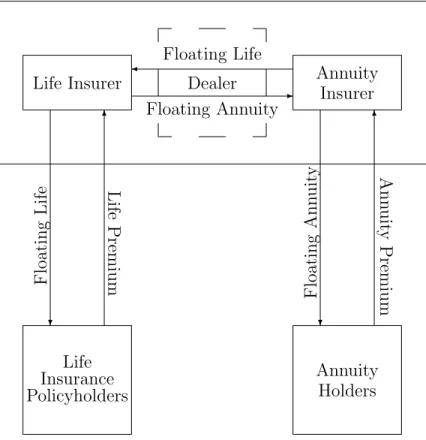
Life Insurer Annuity Insurer Floating Life Dealer Floating Annuity -Life Insurance Policyholders Annuity Holders ? 6 ? 6 Floa ting Life Life Premium Floa ting Ann uit y Ann uit y Premium

Figure 2.2: Mortality Swap Diagram.

survivors in the annuity writer’s specified portfolio of annuities. If, for example, mortality improves, the life insurer pays the annuity writer but it has a gain on its own life insurance policies. There are no other swap payments. Figure 2.2 illustrates the mortality swap cash flows.

2.4.2 Mortality Swap Design

In order to keep the notation fairly simple, I assume that all of the lives in the life insurance portfolio are subject to the same mortality table, denoted by (x), for pricing purposes. At time 0 we have a portfolio of `x lives each insured for an amount f. The random number

of survivors3 _{to age} _x₊_k _{is denoted} _`

x+k. The number of deaths in the year (k, k + 1)

is dx+k = `x+k −`x+k+1. The distribution of dx+k is binomial with parameters m = `x

3_{This is a slight abuse of standard actuarial notation in which} _`x

+k denotes the expected number of

(35)

life insurer’s aggregate death benefit payment in year k + 1 amounts to f dx+k. At time

0, the expected value is E(f dx+k) = f m(kpx −k+1px). The insurer’s risk is that actual

life insurance benefit payments exceed the expected value and so it swaps, agreeing to pay annuity payments (defined below) in exchange for a payment in year k+ 1. The payment from the swap is

f(dx+k−E(dx+k))+ =        f(dx+k−E(dx+k)) if dx+k>E(dx+k) 0 otherwise for k = 0,1, . . . . (2.3) The swap payment limits the net aggregate life insurance benefit from the life insurer to the expected value in each year. Of course, there is a price: The life insurer must provide annuity swap payments when the annuity writer needs them.

The annuity writer pays a benefit b per year to each survivor of an initial cohort of `y

lives all subject to the same table at time 0 (but usually different from the lives on which the life insurance is written). The distribution of `y+k is binomial with parameters m =`y and

q =kpk. The total benefit paid at time k is b`y+k and the annuity writer needs relief when

it exceeds its expected value. This defines the life insurer’s swap payment to the annuity writer: b(`y+k−E(`y+k))+ =        b(`x+k−E(`x+k)) if `y+k>E(`y+k) 0 otherwise for k= 0,1, . . . . (2.4) This is the net cash flow the annuity writer pays in the year (k, k+ 1):

4_{In Section 4.5 in Chapter 4, I show how to model the shift of the selected mortality table by using a}

(36)

Annuity benefits b`y+k

To the life insurer f(dx+k−E(dx+k))+

From the life insurer b(`y+k−E(`y+k))+

Total                        b`y+k if dx+k ≤E(dx+k), `y+k ≤E(`y+k) b`y+k+f(dx+k−E(dx+k)) if dx+k >E(dx+k), `y+k≤E(`y+k) bE(`y+k) if dx+k ≤E(dx+k), `y+k >E(`y+k) bE(`y+k) +f(dx+k−E(dx+k)) if dx+k >E(dx+k), `y+k>E(`y+k)

Here is the life insurer’s net cash flow in the year (k, k+ 1): Death benefits f dx+k

From annuity writer f(dx+k−E(dx+k))+

To annuity writer b(`y+k−E(`y+k))+ Total                        f dx+k if dx+k ≤E(dx+k), `y+k ≤E(`y+k) fE(dx+k) if dx+k >E(dx+k), `y+k≤E(`y+k) f dx+k+b(`y+k−E(`y+k)) if dx+k ≤E(dx+k), `y+k >E(`y+k) fE(dx+k) +b(`y+k−E(`y+k)) if dx+k >E(dx+k), `y+k>E(`y+k)

In each year the swap rearranges the sum of annuity and life insurance benefit payments. The sum is always b`y+k+f dx+k, but the parties swap adverse outcomes. They need not

swap all of their business. The swap contract could be adjusted so that the swap payment triggers are higher than the expected values, for example, or the contract could specify upper bounds on the annual swap payments.

The underlying portfolios of insured lives and annuitants should be selected so that they are subject to the same general mortality change factors. Change factors can move mortality either way. The 1918 flu epidemic is an example which, although the effects varied by age, had a negative impact across populations. Providing pure water and sanitary sewers in

(37)

had a positive effect across populations.

2.4.3 One-Factor Wang Transform

Cairns et al. (2006) discuss a theoretical framework for pricing mortality derivatives and valuing liabilities which incorporate mortality guarantees. Their stochastic mortality models require certain reasonable criteria in terms of their potential future dynamics and mortality curve shapes. Mortality changes in a complex manner, influenced by socioeconomic factors, biological variables, government policies, environmental influences, health conditions and health behaviors. Not all of these factors improve with time and, moreover, opinions on future mortality trends vary widely (Buettner, 2002; Hayflick, 2002; Goss et al., 1998; Rogers, 2002). Even if we could settle on a such a dynamic framework, estimation of the parameters may be very difficult. I take a different, static approach.

Wang (1996, 2000, 2001) has developed a method of pricing risks that unifies financial and insurance pricing theories. This method can be used to price mortality bonds (Lin and Cox, 2005). Now I apply this method to mortality swaps. Consider a random payment X paid at time T. If the cumulative distribution function is F(x), then a distorted or transformed distribution F∗(x) is determined by parameter λ according to the equation

F∗(x) = Φ[Φ−1(F(x))−λ]. (2.5) where Φ(x) is the standard normal cdf. The idea is to determine λ so that the time 0 price of X is its discounted expected value using the transformed distribution. Then the formula for the price is

vTE∗(X) =vT Z

(38)

where vT the discount factor determined by the market for risk free bonds at time 0. Thus,

for an insurer’s given liabilityX with cumulative density functionF(x), the Wang transform will produce a risk–adjusted density function F∗(x). The mean value underF∗(x), denoted by E∗[X], is the risk–adjusted fair-value of X at time T. Wang’s paper describes the utility of this approach. It generalizes well known techniques in finance and actuarial science. My idea is to use observed annuity prices to estimate the market price of risk for annuities, then use the same distribution to price the annuity side of a mortality swap. For the life insurance side I use the same idea. Term life insurance prices to determine the market price of risk in the life insurance market, giving us the appropriate distribution for pricing the life insurance side of the swap.

The Wang transform is based on the idea that the life insurance or annuity market price takes into account the uncertainty in the mortality table, as well as the uncertainty in the lifetime of a life insured or an annuitant once the table is given. The market price of risk does not and need not reflect the risk in interest rates because I am assuming that mortality and interest rate risks are independent. Moreover, I am assuming that investors accept the same transformed distribution and independence assumption for pricing mortality swaps.

The Wang transform is an equilibrium model that can recover the CAPM model. Under the normal distribution assumption, the market price of risk of an asset in the classical CAPM, λ= [E(r)−rf]/σ, is the excess return per unit of volatility. For insurance risks, it

is the risk load per unit of volatility. The Wang transform takes the equilibrium perspective of the CAPM model. If the return of an asset or risk r is normally distributed with mean

µ and standard deviation σ, then the transformed distribution is also normal with mean

µ∗ =µ−λσ and standard deviation σ∗ =σ.

Proof. If r is normal with mean µand variance σ2_{, then}

F(r) = Φ r−µ σ .

(39)

F∗(r) = Φ[Φ−1(F(r)) +λ] = Φ r−µ σ +λ = Φ r−(µ−λσ) σ .

That is, the transformed distribution preserves the normal distribution with mean

µ∗ =µ−λσ (2.7)

and standard deviation σ∗ =σ.

In equilibrium, I expect that the risk-adjusted return µ∗ equals to the risk free rate rf.

Therefore I can rewrite equation (2.7) as

λ= µ−µ

∗

σ =

µ−rf

σ . (2.8)

This is the market price of risk in the CAPM. Moreover, the Wang transform can reproduce the Black–Scholes model with lognormally–distributed assets (Wang, 2002).

The Wang transform has a more desirable property than the CAPM. The CAPM cannot be applied to the situation when the distributions are not normally distributed. So it limits the CAPM’s application in the insurance area where insurance loss distributions are skewed. Contrast to that of the CAPM, the cumulative distribution function FX(x) in the Wang

transform can be some distributions other than normal distributions.

Market price of risk

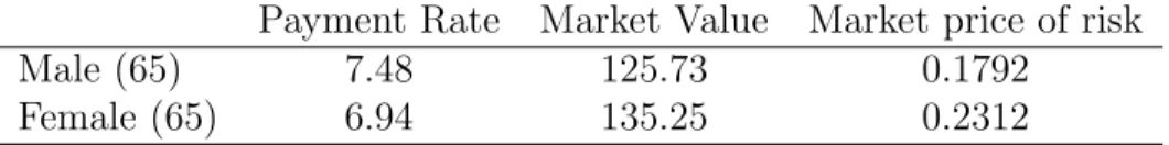
For the annuity distribution function Fa(t) = tq65, I use the 1996 IAM 2000 Basic Table for

a male life age sixty–five. Then assuming an expense factor equal to 4 percent, I use the 1996 market quotes of qualified immediate annuities (Kiczek, 1996) and the US Treasury

(40)

yield curve on December 30, 1996 to get the market price of risk λa by solving the following

equation5 _{numerically for}_λ_:

1000(1−0.04) = 7.48

∞ X

j=1

vj/12[1−Fa∗(j/12)] (2.9)

The variable vj/12 is the discount factor at time 0 for a payment of 1 after j/12 years. And

[1−F_a∗(j/12)] is the survival probability usually denotedj/12p65, but using the transformed

distribution. This has to be solved numerically for λa.

Thus I determine the market price of risk for annuitants is λa = 0.2134. I think of

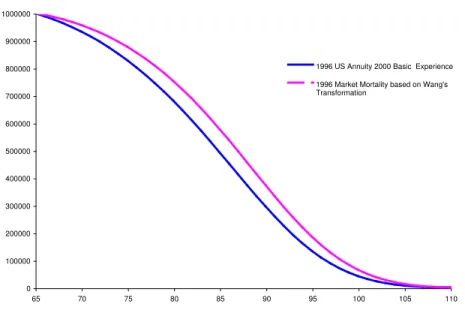
the 1996 IAM 2000 Basic Table as the actual or physical distribution, which requires a distortion to obtain market prices. Figure 2.3 shows the graphs of Fa(t) and Fa∗(t). The

distorted distribution lies to the right and above the physical distribution. This indicates that the market view of annuitant mortality is that it will improve relative to the base table.

Similarly, for the life insurance distribution function Fl(t) = tq35, I use the 1990-95 SOA

Life Insurance Basic Table for a male life age thirty–five. A.M.Best (1996) reports market quotes for both preferred non-smokers and standard smokers. The 1990-95 SOA Basic Table is created based on a mixture of smokers and non-smokers. I calculate a weighted average of term life insurance prices ($507.48) using weights based on the incidence of smoking in the US population as reported by the Center for the Disease Control6 _{in 1995. Assuming an}

expense factor equal to 10 percent, I use the 1996 average market quotes of ten–year level $250,000 term life insurance (A.M.Best, 1996) based on 97 companies and the US Treasury yield curve on December 30, 1996 to get the market price of risk λl = 0.1933 by solving the

5_{The analogous equations in Lin and Cox (2005) are incorrect, although the solutions to the equations}

as stated here, are correct.

6_{Source: www.cdc.gov. About 57 percent former and current male smokers and 43 percent male}

(41)

0 100000 200000 300000 400000 500000 600000 700000 800000 900000 1000000 65 70 75 80 85 90 95 100 105 110

1996 US Annuity 2000 Basic Experience 1996 Market Mortality based on Wang's Transformation

Figure 2.3: The result of applying the Wang transform to the survival distribution based on 1996 IAM experience for males age 65 and prices from Kiczek (1996).

following equation: 507.48×(1−0.10) = 250,000 9 X k=0 vk+1[F∗(k+ 1)−F∗(k)] (2.10)

where vk+1 is the discount factor for a payment after k+ 1 years. A positive life insurance

market price of risk means the market anticipates improved mortality for insured lives, relative to the base table.

Mortality Swap Pricing

I can price each side of the swap now. This will allow me to determine factors b and f

for which the two market prices are equal so no cash is paid by either party to initate the contract; they make only contractual swap payments.

(42)

The market price of the paymentf(dx+k−E(dx+k))+for yearkis its discounted expected

value fE∗[(dx+k − E(dx+k))+]. The “*-distribution” of dx+k is binomial with parameters

m=`x and q=F∗(k+ 1)−F∗(k).7 For large m (over 20 is often suggested), the binomial

distribution is approximately normal and I am thinking of portfolios of hundreds of lives. Thus, to a very good approximation,

E∗[(dx+k−E(dx+k))+]≈σkE[(X−xk)+]

where X is a standard normal variable, µk =mq and σk = p

mq(1−q) are the mean and standard deviation of dx+k and

xk =

E(dx+k)−µk

σk

.

For a standard normal variable X, there is a formula for this (Lin and Cox, 2005):

E[(X−x)+] =φ(x)−x[1−Φ(x)] (2.11)

where φ(x) = Φ0(x) = e−x

2_/₂

√

2π . Thus we can calculate the market price of the life insurance

benefit swap payments as

f ∞ X k=0 vk+1E∗[(dx+k−E(dx+k))+] =f ∞ X k=0 vk+1σk[φ(xk)−xk[1−Φ(xk)]]. (2.12)

I apply this same technique to calculate the market value of the annuity benefit swap pay-ments. I only change the definitions of µk and σk.

b ∞ X k=0 vk+1E∗[(`y+k−E(`y+k))+] =b ∞ X k=0 vk+1σk[φ(xk)−xk[1−Φ(xk)]] (2.13)

The distribution of`y+k is binomial withm=`y andq = 1−F∗(k). The mean are standard

(43)

xk =

E(`y+k)−µk

σk

.

I calculate these values for a 10–year swap, usingm = 10,000 lives in the annuity and life insurance portfolios. The market value of the life insurance payments, for a death benefit of $1,000,000, is $52,758. This is about 1.6 percent of the net term life insurance premium.

For the annuity payment side of the swap, the market value per one dollar of annual benefit, again for 10,000 lives, is $1,690. To adjust the average amount of insurance f per term policy to make each side of the swap have the same price, we have

1,690 =f 52,758

100,000

or f = 3,203. Thus for each dollar of annual annuity benefit we must have $3,203 of death benefit to make the prices equal at time 0. Then each party will have the benefit of natural hedging for 10 years. Even though the prices are equal at time 0, the mortality may move one way or the other so that the future market value favors one party. The swap has to be revalued each year to properly reflect each company’s position as it may be either an asset or liability.

2.5 Conclusions and Discussion

Natural hedging utilizes the opposite reaction of life insurance and annuities to the same mortality change to stabilize aggregate cash outflows. My empirical evidences suggest natural hedging is an important factor contributing to annuity price differences after I control for other variables. These differences become more significant for those insurers selling relatively more annuity business. I expect that life insurers may reach the same conclusion.

(44)

if they reduce their exposure by pooling individual mortality risk and by balancing their annuity positions against their life positions (Dowd et al., 2004). Natural hedging is feasible and mortality swaps make it available widely.

I show how to design a mortality swap between a life insurer and annuity writer to create a natural hedge. Compared with traditional reinsurance and other derivatives, such as mor-tality bonds, mormor-tality swaps may be arranged at possibly lower costs and in a more flexible way to suit diverse circumstances. Thus, there are good reasons to anticipate increased activity in mortality swaps between life insurers and annuity insurers.

(45)

3

Securitization of Mortality Risks in Life

Annuities

Securitization with payments linked to explicit mortality events provides a new investment opportunity to investors and financial institutions. Moreover, mortality-linked securities provide an alternative risk management tool for insurers. The purpose of this paper is to study the securitization of mortality risks, especially the longevity risk inherent in a portfolio of annuities or in a pension plan.

(46)

3.1 Introduction

Securities with mortality risk as a component have been around a long time. These securities arise as securitization of portfolios of life insurance or annuity policies. The risks underlying a life insurance or annuity portfolio include interest rate risk, policyholder lapse risk, as well as mortality or longevity risk. In these transactions, the positive future net cash flow from the policies is dedicated to pay the bondholders. Therefore, they are similar to asset securitization. Cummins (2004) surveys recent life insurance securitization transactions, including these asset-type securities.

However, securitization ofpure mortality or longevity risk is a recent and potentially im-portant innovation in financial markets. Pure mortality or longevity securitization is more like property-linked catastrophe bonds than the common asset-type life insurance securitiza-tion. This is because, like that of a property-linked catastrophe bond based on earthquake or hurricane losses, the payment of a mortality security is subject only to a well-defined risk. In the case of a mortality bond, the event might be a sudden spike in death rates, which may be caused by a flu epidemic.

Catastrophes impose a big potential problem for a life insurer’s solvency since fatalities from natural and man–made disasters may be tremendous. For example, the earthquake and tsunami in southern Asia and eastern Africa in December 2004 killed 182,340 people and resulted in 129,897 missing (Guy Carpenter, 2005). Although most of the victims did not own life insurance, the life insurance industry may not have enough capacity to cover this type of catastrophe losses if such an event were to occur in a more economically developed region where most people buy life insurance. Cummins and Doherty (1997) noted that “a closer look at the industry reveals that the capacity to bear a large catastrophic loss is actually much more limited than the aggregate statistics would suggest.” Securities linked to catastrophe death risk, such as the Swiss Re bond, are discussed in Chapter 4.

This paper focuses on the other side of mortality risk — longevity risk. Although mor-tality improves over time, future rates of improvement are uncertain. At the same time

(47)

US, defined benefit pension plans are converting to defined contribution plans. Proposed Social Security reforms further shift mortality risk to individuals. Thus, there should be an increased demand for individual annuities. As demand for annuities increases, the annuity insurers’ need for risk management of potential mortality improvements will increase.

As a new risk management tool, mortality securitization enhances the capacity of the life insurance industry by transferring its catastrophic losses to financial markets. Jaffee and Russell (1997) and Froot (2001) argue that insurance securitization offers a potentially more efficient mechanism for financing catastrophe losses than conventional insurance and reinsurance. Securitization brings more capital and provides innovative contracting features for the life insurance industry to bear potential mortality shocks, thus avoiding the market disruptions caused by disruptive reinsurance price and availability cycles. Moreover, because mortality securities may be uncorrelated with financial markets, they provide a valuable new source of diversification for market participants (Cox et al., 2000; Litzenberger et al., 1996; Canter et al., 1997). Finally, Cummins (2004) categorizes securitization as arbitrage opportunities or new classes of risk that enhance market efficiency. This paper proposes a feasible way to securitize longevity risk.

In section 3.2, I describe securitization of longevity risk with a mortality bond or a mortality swap. In section 3.3, I illustrate how insurers (or reinsurers or pension plans) can use mortality–based securities to manage longevity risk. In section 3.4, I show how good is the hedge provided by my proposed mortality bond. In section 3.5, I describe the difficulties arising in making mortality projections. I discuss annuity data, including the Individual Annuity Mortality tables and the Group Annuity Experience Mortality (GAEM) reports from Reports of the Transactions of the Society of Actuaries (TSA). Section 3.6 is for discussion and conclusions.

(48)

3.2 Mortality Securitization

I propose a new type of mortality bond which is similar to the Swiss Re deal discussed in Section 4.3.1 but focused on longevity. The structure is similar to other deals. Generally, the life-based securitizations follow the same structure as the so called catastrophe-risk bonds. There have been more than thirty catastrophe bond transactions reported in the financial press and many papers written about them. Mortality bonds are different in several impor-tant ways. For example, deviation from mortality forecasts may occur gradually over a long period, as opposed to a sudden property portfolio loss. However, in both transactions, costs are likely to be high relative to reinsurance on a transaction basis.

In both transactions, the insurer (reinsurer or annuity provider) purchases reinsurance from a special purpose company (SPC). The SPC issues bonds to investors. The bond contract and reinsurance convey the risk from the annuity provider to the investors. The SPC invests the reinsurance premium and cash from the sale of the bonds in default-free securities. I will show how this can be set up to allow the SPC to pay the benefits under the terms of the reinsurance with certainty.

3.2.1 Example

As an example of a mortality securitization, consider an insurer1 _{that must pay immediate}

life annuities to `x annuitants2 all aged x initially. Set the payment rate at 1,000 per year

per annuitant. Let`x+tdenote the number of survivors to yeart. The insurer pays 1,000`x+t

to its annuitants, which is random, as viewed from time 0. I will define a bond contract to hedge the risk that this portion of the insurer’s payments to its annuitants exceeds an agreed upon level.

The insurer buys insurance from its SPC for a premium P at time 0. The insurance

1_{The “insurer” could be an annuity writer, annuity reinsurer or private pension plan. The counter party}

could be a life insurer or investor.

2_{The security could be based on a mortality index rather than an actual portfolio. This will avoid the}

(49)

excess of the actual payments over the trigger. In year t the insurer pays amount 1000`x+t

to its annuitants. If the payments exceed the trigger for that year, it collects the excess from the SPC, up to a maximum amount. Let us say that the maximum is stated as a multiple of the rate of annuity payments 1000C. Thus in each yeart= 1,2, . . . , T the insurer collects the benefit Bt from the SPC determined by this formula:

Bt=                1000C if `x+t > Xt+C 1000(`x+t−Xt) if Xt < `x+t≤Xt+C 0 if `x+t ≤Xt (3.1)

The insurer specifies the annuitant pool in much the same way that mortgage loans are identified in construction of a mortgage–backed security. The insurer’s cash flow to annuitants 1000`x+t at timet is offset by positive cash flow Bt from the insurance:

Insurer’s Net Cash Flow = 1000`x+t−Bt (3.2)

=                1000(`x+t−C) if `x+T > C +Xt 1000Xt if Xt < `x+t≤C+Xt 1000`x+t if `x+t ≤Xt

For this structure, there is no basis risk in the reinsurance. Basis risk arises when the hedge is not exactly the same as the reinsurer’s risk. The mortality bond covers the same risk, so there is no basis risk. This is in contrast to the Swiss Re deal, which is based on a population index rather than a portfolio of Swiss Re’s life insurance polices (or its clients’ policies). While there is no basis risk, the contract does not provide full coverage. I will study the distribution of the present value of the excess later.