Variance: The Case with Independent Noise
∗OLE E. BARNDORFF-NIELSEN
Department of Mathematical Sciences, University of Aarhus
PETERREINHARDHANSENy
Department of Economics, Stanford University
ASGER LUNDE
Department of Marketing, Informatics and Statistics, Aarhus School of Business
NEILSHEPHARD
Nuffield College, University of Oxford
This Draft: November 15, 2004
Abstract
We consider kernel-based estimators of integrated variances in the presence of independent market microstructure effects. We derive the bias and variance properties for all regular kernel-based estimators and derive a lower bound for their asymptotic variance. Further we show that the subsample-based estimator is closely related to a Bartlett-type kernel estimator. The small difference between the two estimators due to end effects, turns out to be key for the consistency of the subsampling estimator. This observation leads us to a modified class of kernel-based es-timators, which are also consistent. We study the efficiency of our new kernel-based procedure. We show that optimal modified kernel-based estimator converges to the integrated variance at rate m1/4,where m is the number of intraday returns.
JEL Classification: C13, C22.
Keywords: Quadratic Variation, Market microstructure noise, Integrated variance, Kernel-based realized variance, Realized variance, Realized volatility.
∗We thank Yacine Ait-Sahalia, Ulrich M¨uller, and Joe Romano for valuable comments.
yCorresponding author: Peter Reinhard Hansen, Stanford University, Landau Economics Building, 579 Serra Mall,
1. Introduction
In the last five years substantial improvements in our understanding of and ability to forecast finan-cial volatility has been possible through the harnessing of high frequency finanfinan-cial return data. The key developments have been the use of estimators of quadratic variation, (e.g. Andersen, Bollerslev, Diebold & Labys (2003) and Barndorff-Nielsen & Shephard (2002)) and making sense of their prop-erties when applied to 5 to 30 minute return data. A weakness with existing methods is their inability to deal with market microstructure effects whose effects are key when we use returns recorded over very short time intervals. Interesting recent innovations that improve our comprehension of this topic include A¨ıt-Sahalia, Mykland & Zhang (2003), Bandi & Russell (2004), Hansen & Lunde (2004a, 2004c), and Zhang, Mykland & A¨ıt-Sahalia (2004).
The problem of estimating the quadratic variation is, in some ways, similar to the estimation of the long-run variance in stationary time-series. So it is not surprising that the literature has studied estimation methods that are well-known from the literature on covariance estimation, including pre-whitening methods, likelihood-based estimators, and kernel estimators. For example, the popular realized variance (RV) is analogous to the sum-of-squares variance estimator. Because the RV is sensitive to market microstructure noise it is recommended to use sparse sampling in practice, and the optimal sampling frequency is derived in Bandi & Russell (2004) and Zhang et al. (2004). The moving average filter used by Andersen, Bollerslev, Diebold & Ebens (2001) and the autoregressive filter used by Bollen & Inder (2002), are estimators that use pre-whitening techniques, and Bandi & Russell (2004) analyze optimal sampling of pre-whiten series. Likelihood-like estimators include the maximum likelihood estimators of A¨ıt-Sahalia et al. (2003) who use a homogeneous diffusion model framework and the GMM estimator of Oomen (2004b) who use a pure jump model. The subsample estimator of Zhang, Mykland & A¨ıt-Sahalia (2002) stands out as the only existing non-parametric estimator that is consistent, and its analog for estimation of the long-run variance was introduced by Carlstein (1986).
Our focus will be on kernel-based estimators. This literature was started by Zhou (1996) who proposed a particular kernel estimator, which only incorporates the first-order autocovariance. This suffices for unbiasness under “independence noise” where the population value of higher-order au-tocovariances are zero. Hansen & Lunde (2004a, 2004c) primarily use kernel-based estimators to characterize properties of market microstructure noise. Hansen & Lunde (2004a) use the estimator of Zhou (1996) to construct a test for “independent noise” and provide empirical evidence of time-dependence in the noise when return data are sampled at ultra high frequencies, such as every few
ticks. Hansen & Lunde (2004c) analyze the properties of realized variance under general assump-tions about the noise and derive a particular unbiased kernel estimator, that can be used to uncover the time-dependence in the noise. Thus, the existing literature on kernel estimators has either fo-cused on that based on the first-order autocovariance, see Zhou (1996), or used particular unbiased kernels to analyze and characterize features of market microstructure noise, see Hansen & Lunde (2004a, 2004c).
In this paper we provide the first systematic study of kernel-based estimators of the integrated variance in the presence of market microstructure noise. We derive the optimal kernel-based esti-mator under an assumption that the noise is without memory and independent of the efficient price, an assumption which is empirically reasonable at moderate time scales such as 1-minute returns in highly liquid markets. Even though second and higher-order autocovariance are known to be zero under this assumption, we show that it pays off to estimate these. This makes it possible to derive kernel-based estimators that are far more precise than is that of Zhou (1996). However, we also show that there does not exist a consistent regular kernel-based estimator, so there is a limit to the precision of regular kernel-based estimators. Interestingly, we show that the consistent subsampling estimator of integrated variance by Zhang et al. (2004) is closely related to a particular kernel-based estimator. Importantly, it turns out that the difference between regular kernel estimators and the subsampling estimator, generated by end effects, is crucial for the consistency of the subsampling estimator. This observation allows us to propose a modified kernel-based estimator which is consis-tent. We study the efficiency of the new class of estimators and find its rate of convergence to be the optimal rate, m1/4, where m is the number of intraday returns, see Gloter & Jacod (2001a, 2001b). So this rate is as good as the rate that can be obtained by a maximum likelihood estimator under more restrictive distributional assumptions for the noise.
In Section 2 we detail our assumptions about the noise, efficient price process and sampling scheme. In Section 3 we detail one of our main contributions, a systematic analysis of the properties of regular kernels. In Section 4 we related subsampling estimators to Bartlett-style regular kernels, and we see the difference is due to end conditions. In Section 5 we introduce the new modified kernel estimator and study its properties. In Section 6 we draw some conclusions. A lengthy Appendix provides the proofs of the results given in the paper.
2. Assumptions
2.1. Price Process and Noise
Without loss of generality we assume that the observed price process is given by
p(t)= p∗(t)+u(t), t∈[0,T ], (1)
where we label p∗ as the efficient price process and u as the noise process. We assume that the efficient price is given from the simple diffusion model, d p∗(t) = σ (t)dw(t), where w(t) is a standard Wiener process that is independent of{σ2(t)}tT=0,and we make the following assumptions about the noise process.
(N) The noise process u has mean zero, varianceω2≡ E [u2(t)]<∞,and kurtosisκ ≡E [u4(t)]/ω4 <∞. Moreover, u(s)⊥⊥ p∗(t)for all s,t ∈[0,T ] and u(s)⊥⊥u(t)for all s 6=t.
There is plenty of empirical evidence against(N) when prices are sampled at ultra-high fre-quencies, such as every few ticks, see Hansen & Lunde (2004a, 2004c) who show that u is neither time-independent nor independent of p∗.On the other hand, Hansen & Lunde (2004a) also note that there is little evidence against (the implications of)(N)when prices are sampled at more moderate frequencies such as every 15 ticks. Because the analysis become much more complicated if u is time-dependent, all our results are derive using (N).So our results may not apply to tick-by-tick data. The advantage of our strategy is that it will produce a clear cut analysis of the core issues of kernel-based estimators.
Equation (1) may be viewed as a (Beveridge-Nelson type) decomposition, where p∗ and u represent the persistent component and transitory component, respectively. So the volatility of p(t +s)− p(t) is well approximated by that of p∗(t +s)− p∗(t) when s is large. Thus, the volatility of p∗is the appropriate object of interest, even for the reader who is exclusively interested in the volatility of p (whether p is autocorrelated or not).
Without loss of generality we consider the unit interval of time, [0,1], that is divided into m sub-intervals ti,m−ti−1,m,i =1, . . . ,m, (t0,m =0 and tm,m =1).The innovations in p∗, p,and u over each of the sub-intervals are defined by, for i =1,2, . . . ,m,
yi∗,m ≡ p∗(ti,m)−p∗(ti−1,m), yi,m ≡ p(ti,m)−p(ti−1,m), ei,m ≡u(ti,m)−u(ti−1,m). We will refer to yi∗,mand yi,mas intraday returns, and we note that yi,m =yi∗,m+ei,m.
We define the integrated variance
IV ≡
Z 1 0
σ2(s)ds,
which is the object we would like to estimate. Our assumptions about the efficient price implies that IV = Pmi=1σi2,m,whereσ2i,m ≡ var(yi∗,m),1i = 1, . . . ,m.In fact we have that y∗
1,m, . . . ,ym∗,m are independent and Gaussian distributed, yi∗∼ N(0, σ2i,m),(conditionally on{σ2(s)}1s=0). Throughout we make the following assumptions about the volatility path.
(V) The volatility is (pathwise) continuous on [0,1], strictly positive, and satisfies
m−1/2 m X
i=1
|σr(si,m)−σr(s˜i,m)| =o(1),
for some r > 0 (equivalently for all r > 0)2 where si,m ands˜i,m are arbitrary points in the interval [ti−1,m,ti,m],i=1, . . . ,m.
2.2. Sampling Scheme
We make the following assumption about the sampling times, t0,m,t1,m, . . . ,tm,m,where we use⌈a⌉ to denote the smallest integer greater than or equal to a.
(T) It holds that sups∈[0,1]|t⌈sm⌉,m −τ (s)| = o(m−1), where τ is continuous and differentiable function,τ (0)=0 andτ (1)=1,and 0< τ′(s) <∞for all s ∈[0,1].
The special case where the price observations are equidistant in time, corresponds to ti,m =i/m, in which case τ (s) = s and τ′(s) = 1.Mykland & Zhang (2005) use a similar framework for sampling times, see also Barndorff-Nielsen & Shephard (2005). Given(T)we have the following result that corresponds to Assumption A.v in Mykland & Zhang (2005).
Lemma 1 Given(T)it holds that
lim m→∞1≤supi≤m ti,m−ti−1,m 1/m −τ′( i m) =0.
1All population moments are made conditional on the stochastic volatility process,{σ2(s)}1
s=0,which defines our
object of interest. To simplify notation we use the convention E(·)≡E(·|{σ2(s)}s1=0) ,and similar for var(·),and cov(·). 2See Barndorff-Nielsen & Shephard (2003).
Also key for our analysis is the (time-deformed) integrated quarticity,
IQ≡
Z 1 0
τ′(s)σ4(s)ds,
and it holds that mPmi=1σi4,m =IQ+o(1),whereσ4i,m ≡(σ2i,m)2,see Lemma A.2 in the appendix. An interesting sampling scheme is that whereτ (s)is the solution toR0τ (s)σ2(r)dr =s·IV,such thatσ2i,m = IVm for all i = 1, . . . ,m.We refer to this as Business Time Sampling (BTS), see Oomen (2004a, 2004b). As noted by Hansen & Lunde (2004a), BTS minimize IQ≡R01τ′(s)σ4(s)ds =
IV2,as the implicit function theorem shows thatτ′(s)= IVσ2(s)under BTS. (T′) Condition(T)holds withτ′(s)= IVσ2(s).
3. Properties of Regular Kernel-Based Estimators
We consider the family of RV-estimators{RVw: w∈Rm}given by
RVw ≡w0γˆ0+ m−1 X h=1 wh(γˆ−h+ ˆγh), whereγˆ±h≡ m−h X i=1 yiyi+hfor h =0, . . . ,m−1, and we call this the class of regular kernels. These types of statistics are familiar from the litera-ture on covariance stationary processes, where they are used to estimate the long-run variances and covariances. Leading examples of this include Newey & West (1987) and Andrews (1991). This theory is not directly applicable here as our in-fill asymptotics is entirely different from the con-ventional setup. Further, the market microstructure noise in our problem will induce a particular autocovariance structure that we will use to characterize the kernels that provide good estimates of the IV.
Examples of kernel-based estimators for estimation of integrated variance from high-frequency data include those by Zhou (1996) (ωh =0 for h≥2),Hansen & Lunde (2004c)(ωh=(m+h)/m for h ≤ ⌈ρm⌉0≤ ρ <1),and Hansen & Lunde (2003, 2004b) (Bartlett kernel). Interestingly, we will show in Section 4 that the subsample-based estimator of Zhang et al. (2004) is almost identical to a Bartlett-type kernel estimator. However, the feature that makes the subsample estimator dis-tinct from any kernel estimator turns out to be very informative about the estimation problem, and suggests a modified class of kernel estimators. We will spell this out in Section 5.
Since any kernel-based RV is a linear combination ofγˆ ≡(γˆ0,2γˆ1, . . . ,2γˆm−1)′, we can study
For any m×m matrix A= {ai j}mi,j=1and any function, f,that is integrable on [0,1] we define the operator f 7→I(A, f),which yields the m×m matrix with elements
{I(A, f)}im,j=1≡Ai j Z 1 0 ψι i j(s)f(s)ds, whereιi j ≡ max(i,j)−1 m , and ψρ(s)≡ 1 for s ∈[ρ,1−ρ] 1 2 otherwise.
When f(s)=c for all s,we write I(A,c)≡I(A, f)and note that I(A,c)=cI(A,1)and that
{I(A,c)}mi,j=1=Ai j(1−ιi j)c.
Theorem 2 Given(N), (V)and(T), then E(γˆ′)=(IV+2mω2,−(m−1)2ω2,0, . . . ,0)and
cov(γˆ)=I(A, ω4)m−2ω4C+ω2I(B, σ2)+I(C, σ4τ′)m1 +Ho(m1),
where the m×m matrices (assumingκ=3)are given by
A = 12 −16 4 0 · · · −16 28 −16 4 . .. 4 −16 24 −16 . .. 0 4 −16 24 . .. .. . . .. . .. . .. ... , B= 8 −8 0 0 · · · −8 16 −8 0 . .. 0 −8 16 −8 . .. 0 0 −8 16 . .. .. . . .. ... ... ... , C = diag(2,4,4,4, . . .), H=diag(1,1,2,3,4, . . .).
Remark 1 The matrix H has a lower-right element of m−1,such that Ho(m1)is not o(m1).However, for the first q autocovariances, where q is a fixed number the reminder term for this submatrix of cov(γˆ)is simply o(m1),because all terms of this submatrix are at most o(mq) =o(m1).Later where
we let q =qm → ∞as m → ∞,the last terms is o(qmm).
Remark 2 The variance simplifies considerably under(T′)where IV2=IQ,in which case we have that
where ¯ A≡I(A,1)= 12 −16mm−1 4mm−2 0 · · · −16mm−1 28mm−1 −16mm−2 4mm−3 . .. 4mm−2 −16mm−2 24mm−2 −16mm−3 . .. 0 4mm−3 −16mm−3 24mm−3 . .. .. . . .. . .. . .. ... ,
and similar forB and¯ C. Thus¯ A¯i j =(1−ιi j)Ai j = m−maxm(i,j)+1Ai j for all i,j =1, . . . ,m.
Remark 3 Theorem 2 is formulated for the case whereκ =3.The result for the general case where
κ is arbitrary, requires the upper left 2×2 submatrix of A to be written as
4κ −4(κ+1)
−4(κ+1) 4(κ+4)
,
whereas all other elements of A are unchanged, see the proof of Theorem 2. Restricting our attention to the case whereκ =3 has no important implication for our analysis, because the bias properties require that ω0, ω1 → 1 as m → ∞,which eliminates theκ-terms in A (since 4κ+4(κ +4)− 8(κ+1)=8 does not involveκ,see Hansen & Lunde (2004a)).
Several results in the existing literature now follow as special cases of Theorem 2. Ifω2 = 0 we have the result by Jacod (1994) and Barndorff-Nielsen & Shephard (2002) that var(RV(m)) = 2IQm1+o(m1),see also Jacod & Protter (1998). Whenω2>0 we have the expressions bias(RV(m))= 2mω2and var(RV(m))
=12mω4+O(1)by Bandi & Russell (2004) and Zhang et al. (2004). More generally we have the following result by Hansen & Lunde (2004a) that var(RV(m)) = (12m − 4)ω4+8ω2IV +2IQ1
m +o(
1
m),and the result by Zhou (1996) that var(RV
(m)
AC1)= (8m−12)ω
4+ 8ω2IV+6IQm1+o(m1),for RVAC(m1)≡ ˆγ0+2γˆ1,which now follows from Theorem 2 as special cases. The interesting aspect of Theorem 2 is that adding estimates of autocovariance terms (that have a population value that is known to be zero) can increase the precision whenever ω2 > 0. The following Corollary contains results for the cases where the second and third autocovariances are included, using weights that minimize the asymptotic variance. For notational convenience we definevρ ≡
Rρ 0 σ
2(s)ds+R1 1−ρσ
2(s)ds and we note thatv h m =σ
2
1+ · · · +σ2h+σm2−h+1+ · · · +σ2m for integers of h.
Corollary 1 Define RVAC(m2)≡ ˆγ0+2γˆ1+ ˆγ2,RVAC(m3) ≡ ˆγ0+2γˆ1+57γˆ2+35γˆ3.Under the assumptions of Theorem 2 both estimators have bias of 2ω2while
var(RVAC(m) 2) = 2mω 4 +4ω2IV+7IQm1 +2ω2(v2 m +ω 2) +o(m1), var(RVAC(m) 3) = 4 5mω 4 +68 25ω 2IV +208 25IQ 1 m +8 21 100ω 2v 2 m +8 12 100ω 2v 3 m + 98 25ω 4 +o(m1). Corollary 1 shows that by adding (a linear combination of) higher-order autocovariances can reduce the variance without affecting the bias (for m sufficiently large), as the higher-order terms (or linear combination of these) have a zero mean and are negatively correlated withγˆ0+2γˆ1,such that adding a proper linear combination will lead to a reduction of the total variance.
The linear combinations of the higher-order autocovariances that were included in Corollary 1, 1γˆ2and75γˆ2+35γˆ3,where chosen in order to minimize the asymptotic variance that is of orderω4m. This also led to a reduction of the variance term that is of order m0(from 8 to 4 and 6825 timesω2IV respectively), whereas the m−1-variance term was increased, and the last observation highlights the need to study all terms in our analysis of kernel-based estimators.
For notational convenience we define IVρ ≡ R1
0 ψρ(s)σ2(s)ds and IQρ ≡ R1
0 ψρ(s)σ4(s)ds,and
we note that IV−IVρ = 12vρ,and that IQ−IQρ = O(ρ),such that 1 m(IQ−IQmh)=O( h m2)=o( 1 m).
Corollary 2 Let w=(w0, . . . , wm−1)′.The bias of RVwis given by
bias(RVw)=(w0−1)IV+(w0−mm−1w1)2ω2m =w′(IVd+2mω2f)−IV,
where d=(1,0, . . . ,0)′and f=(1,−mm−1,0, . . . ,0)′;whereas the variance is given by var(RVw)=V1ω4m+V0ω2+V−1m1 +o(m1), where V1(w)=12w20+ m−1 m w14(7w1−8w0)+ mP−1 j=2 m−j m wj8(3wj−4wj−1+wj−2) − 4 mw 2 0− 8 m mP−1 j=1 w2j, V0(w)=8IVw02+ mP−1 j=1 16IVj mwj(wj−wj−1), and V−1(w)=2IQw 2 0+ mP−1 j=1 4IQj mw 2 j.
Thus, V1 = o(m1) is a necessary condition for the variance of RVw to vanish, and w0 → 1 as m → ∞is clearly required for RVw to be generally consistent for IV.While there are other
V1=o(m1),which appears to be the most stringent requirement. For this reason, we seek the kernel that minimizes V1(w)subject to the constraint thatw0=1.
Theorem 3 (Variance Bound for Regular Kernel-Based Estimators) It holds that w⋆ ≡arg min w∈RmV1(w), subject tow0=1, is given by w⋆ =(1,w⋆′ 2)′where w ⋆ 2≡ −M− 1
22M21and M22and M21are submatrices of
¯ Am−2C= M11 M12 M21 M22 ,
with dimensions(m−1)×(m−1)and(m−1)×1,respectively. Further, it holds that mV1(w⋆)=w⋆′(Am¯ −2C)w⋆ →4, as m → ∞.
Theorem 3 shows that it is not possible to drive the variance of a regular kernel-based estimator to zero, as m → ∞.The result shows that 4ω4is a lower bound for the asymptotic variance. So the existence of a consistent regular kernel-based estimator is ruled out.3 While consistency is clearly important, it is worth noticing that the non-vanishing variance term, 4ω4,is likely to be very small in practice. For example, Hansen & Lunde (2004a) estimateω4to be of an order in the neighborhood of 10−8 for the stocks of the Dow Jones Industrial Average. Consistency is convenient because it justifies theδ-method, such that a central limit theorem (CLT) for log(w′γˆ),say, follows from a CLT
for w′γˆ.Naturally, if 4ω4is negligible relative to var(w′γˆ),the distortions from using theδ-method
to approximate the distribution of log(w′γˆ),say, will be extremely modest. Nevertheless, the mere
existence of consistent estimator – the subsample estimator of Zhang et al. (2004) – does challenge the usefulness of regular kernel-based estimators. So in the following two sections we shall study the subsample-based estimator and a modified class of kernel-based estimators, where the latter is motivated by the relation between the subsample estimator and a particular kernel-based estimator. But first we evaluate how far we can push the precision of regular kernel-based estimators.
Theorem 3 provides a lower bound for the asymptotic variance of regular kernel-based estima-tors, derived from V1.Since the variance also involves the terms, V0and V−1it is unclear whether this bound can be obtained by any kernel. This question is addressed by the following Lemma that gives a simple example of a scheme for w which achieves the lower bound. This estimator is almost 3While consistency does not require the variance to vanish, consistency is indeed ruled out in the present setting,
identical to that introduced to this context by Hansen & Lunde (2003), and later applied by Hansen & Lunde (2004b).
Lemma 4 Consider the Bartlett-type kernel, where the elements of wBare given by w0= mm−1q−q1, wj = q−qj for j =1, . . . ,q, wj =0 for j >q,
wherew0= mm−1w1in order to eliminate the bias. Given(N),(V),and(T′)it holds that
V1=4m1 +O(q12), V0= O(mq), V−1=O(q
2
m),
such that var(RVwB) = 4ω
4 + O(qm2)+O( q m),which tends to 4ω 4 provided that q/m → 0 and q2/m→ ∞as q,m→ ∞.
Since the Bartlett-type kernel in Lemma 4 achieves the lower bound, it is asymptotically efficient in the class of regular kernel estimators.
3.1. Bias Eliminating Regular Kernels Lemma 5 We defineλ≡ω2/IV,
6λ≡(Am¯ −2C)λ2+ ¯Bλ+ ¯Cm1 and 4λ≡(d+2mλf)(d+2mλf)′,
where d and f where defined in Corollary 2. Under the assumptions of Theorem 2 and(T′), we have that MSE(RVw)/IV2=w′(6λ+4λ)w−2w′(d+2mλf)+1.
While Lemma 5 is useful in order to evaluate the MSE for a given kernel estimator, it does not constitute a useful way to define an optimal kernel, such as w⋆ ≡ arg min
wMSE(RVw) = (6λ + 4λ)−1(d+2mλf), because such a kernel would be extremely sensitive to small variations in λ.4
Instead we restrict attention to kernels for which w0 = mm−1w1 andw0 → 1 as m → ∞.These restrictions guarantees that the resulting estimator is asymptotically unbiased, as can we verified from E(γˆ)that was stated in Theorem 2. Note that the Bartlett-type kernel in Lemma 4 satisfies
this criterion. The reason that we do not impose the constraint w0 = 1, is that the MSE may be reduced by allowingw0to be slightly smaller than one, (i.e. trading a small increase in the bias for a reduction of the variance).
4This issue can be understood by considering the kernel given by:w
0=IV/(IV+2ω2m)=1(1+2λm)andwh=0
for h≥1.Forλm=4.5 we havew0=1/10,which is unbiased if indeedλm=4.5,but can be severely biased for other
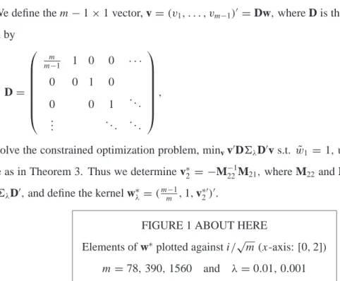
We define the m−1×1 vector, v=(v1, . . . , vm−1)′=Dw,where D is the m−1×m matrix given by D= m m−1 1 0 0 · · · 0 0 1 0 0 0 1 . .. .. . . .. ... ,
and solve the constrained optimization problem, minvv′D6λD′v s.t. w˜1 =1,using the same tech-nique as in Theorem 3. Thus we determine v∗2 = −M−221M21, where M22and M21 are submatrices of D6λD′,and define the kernel w∗λ =(
m−1
m ,1,v∗′2)′.
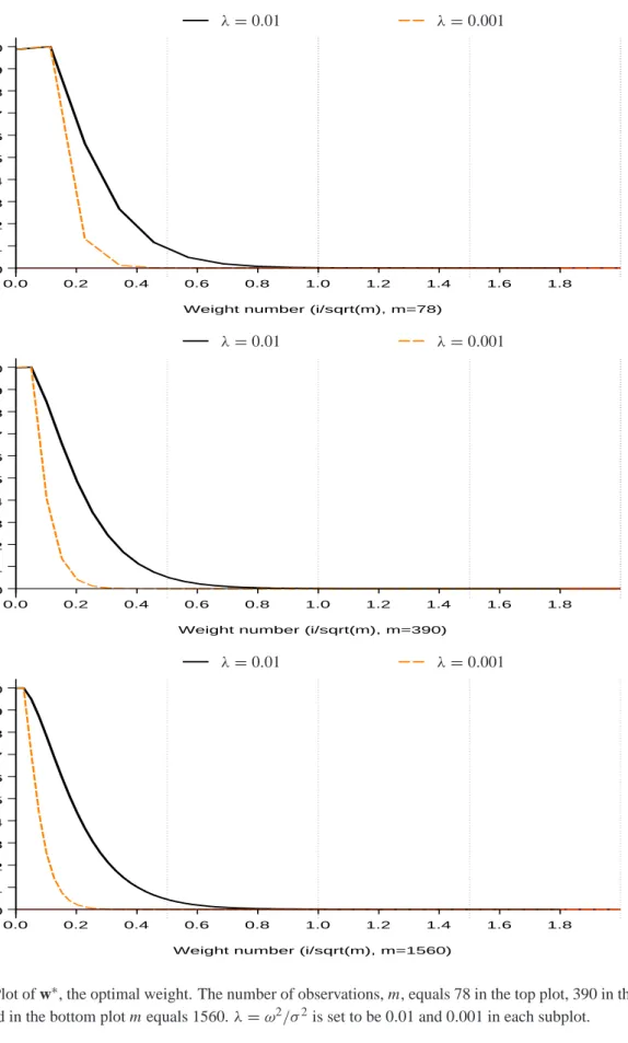
FIGURE 1 ABOUT HERE
Elements of w∗plotted against i/√m(x-axis: [0,2])
m =78,390,1560 and λ=0.01,0.001
Although our kernel is derived under the independent noise assumption, we note that the kernel has some degree of robustness to mild time dependence in the noise process. Time dependence in the noise process causes higher-order covariances to have an expected value that is different from zero, since the kernel above haswi > 0,for i =2,3, . . .it is somewhat capable of capturing this deviation from the indpendence assumption.
The rate at which the variance of RVw∗λconverges to 4ω4can be determined numerically from an
ancillary regression and we find this rate to be m−1/2.We describe the ancillary regressions towards the end of Section 5.
4. Subsample-Based Estimator
Zhang et al. (2004) have proposed a very stimulating subsample-based estimator of integrated vari-ance. In an unpublished paper M¨uller (1993) also studied the use of subsampling to estimate the variability of financial prices. His motivation was the same as Zhang et al. (2004), but his analysis was much less formalized, so we will focus entirely on the contribution from Zhang et al. (2004). The subsample estimator can be constructed from the grid, G ≡ {t0,t2, . . . ,tm},5 and the (non-overlapping) subgrids, Gk j = {tj−1,tj−1+k, . . . ,tj−1+cjk}, for j =1, . . . ,k where cj ≡ j m−j+1 k k ,
and⌊a⌋denotes the largest integer that is smaller than or equal to a.So the subgrids are such that Gk
i ∩Gkj = ∅for i 6= j andG= Sk
j=1Gkj for any k≤m.For each subsample we can calculate the realized variance
RVGk j ≡
X
ti∈Gk j
yt2i,ti+k, where yti,ti+k ≡ pti+k− pti,
with the convention that yti,tj =0 if j >m.The k-subsampling estimator by Zhang et al. (2004) is given by RVsubk = 1k k X j=1 RVGk j − m−mkk+1RVG.
Theorem 6 It holds that
RVsubk =(1−m−mkk+1)γˆ0+ k X h=1 k−h k (γˆ−h+ ˆγh)−k1rk,
where r1≡0 and rk ≡rk−1+(y1+ · · · +yk−1)2+(ym−k+2+ · · · +ym)2for k ≥2.
It is very interesting that the subsample-based estimator is almost identical to the kernel-based estimator that employs the Bartlett-type kernel:
wsubk =(1−m−mkk+1,k−k1,k−k2, . . . ,1k,0, . . . ,0)′. The difference is the presence of rk.
Remark 4 Theorem 6 provide a way to implement the subsampling estimator, as RVsubk (for any k)
can be calculated from the empirical autocovariances and the recursive formula for rk.
Remark 5 The close relationship between RVsubk and kernel-based estimators, stems from the fact
that yti,ti+k =yi+1+ · · · +yi+k,such that RVsubk is simply a linear combination of cross products of
intraday returns, yi,myj,m,i,j =1, . . . ,m,as is the case for all kernel-based estimators. That the subsample estimator is closely related to the Bartlett kernel is perhaps not too surprising, because Bartlett (1950) motivated the Bartlett kernel with the subsampling idea, see also Anderson (1971, p. 512) and Priestley (1981, pp. 439–440). Interestingly Politis, Romano & Wolf (1999) noted that the subsample estimator (of the long-run variance) of Carlstein (1986) is identical to both the moving block bootstrap estimator and the Jackknife estimator in this case, see K¨unsch (1989) and Liu & Singh (1992). Further, the term, k1rk,that makes RVsubk distinct from kernel-based estimators
Remark 6 The really surprising result of Theorem 6 is that 1krk,which is innocuous in the contest of conventional stationary time series, is indeed crucial for the consistency of RVsubk.Zhang et al.
(2004) show that limm→∞var(RVsubk)=0 for a suitable choice of k=km.So 1krk is responsible for the increased precision beyond the lower bound, 4ω4,that we established for kernel-based
estima-tors in Theorem 3. It is interesting here to note the results in M¨uller (2004) that shows that the most ‘robust’ quadratic estimator is not a kernel estimator.
Lemma 7 Given(N)and(V)it holds that
E(rk) = k−1 X h=1 h(σ2h+σ2m+1−h)+4(k−1)ω2, var(1krk) = 4k−k1ω4+O(mk), cov(1krk,bγ′) (=1) ω4(12k−k1/3,−8k−k1,0, . . . ,0).
Here we have used(=1)to denote equality in terms of theω4-terms, while other terms that involve σ2i,mandσ4i,m are omitted as these are O(m−1)and O(m−2),respectively.
Lemma 7 shows that
var(RVsubk) = var(RVwsubk − 1krk)
(1)
= 4ω4+4k−k1ω4−2cov(1krk,bγ′)w
→ 4ω4+4ω4−2(12ω4−8ω4)=0 as k,m→ ∞,
confirming that RVsubk is consistent whereas the Bartlett type estimator is inconsistent. Another result that follows from Lemma 7 is that the bias of RVsubk is given by
bias(RVsubk) = (1− m−mkk+1−1)IV+(1− m−mkk+1−mm−1k−k1)2ω2m− 1kE(rk) = −m−k+1 mk IV− 1 k k−1 X h=1 h(σ2h+σ2m+1−h), (2) which can be verified to be of order O(mmk+k2).Thus bias(RVsubk)=o(1)if k/m =o(1)as k,m →
∞.
5. Modified Kernel-Based Estimators
Having understood the connection between a regular kernel estimator and subsampling and gained an appreciation of why subsampling is consistent, we are now in a position to modify the regular kernel-based estimator to inherit that property. Our hope is to deliver a consistent estimator which is reasonably efficient even in small samples.
For h≥1 we define
zh≡ yh2+2yh(yh−1+ · · · +y1), and z˜h ≡ym2−h+1+2ym−h+1(ym−h+2+ · · · +ym), then it can be shown that
rk = k−1 X j=1 (k− j)zj+ k−1 X j=1 (k− j)˜zj, (see the proof of Lemma 7) such that
RVsubk = (1−m−mkk+1)γˆ0+ k−1 X h=1 k−h k 2γˆh−1krk = (1−m−mkk+1)γˆ0+ k−1 X h=1 k−h k (2γˆh−zh− ˜zh)=w′subkγ˜,
where we use the vector of modified autocovariances estimators,
˜
γ ≡(γˆ0,2γ˜1, . . . ,2γ˜m−1)′, 2γ˜h≡2γˆh−zh− ˜zh, for h ≥1.
Thus inspired by the subsample estimator, we consider a modified class of kernel estimators, given by{ ˜w′γ˜ :w˜ ∈ Rm}.This class of estimators contains at least one consistent estimator of IV.
Theorem 8 gives the properties of the underlyingγ˜. Theorem 8 Given(N), (V)and(T′), it holds that
E(γ˜)=(IV+2mω2,−2(m+1)ω2− 2 mIV,− 2 mIV, . . . ,− 2 mIV) ′ and
cov(γ˜)=cov(γˆ)+ ˜Aω4+m1B˜ω2IV+ m12CIV˜
2 ,
where the upper left q×q sub-matrices ofA˜,B˜,andC are given by˜
˜ Aq = 0 −20 8 0 · · · −20 48 −28 8 . .. 8 −28 40 −28 . .. 0 8 −28 40 . .. . . . . .. . .. . .. . .. , B˜q = 0 −8(2) 0 0 · · · −8(2) 16(2) −8(3) 0 . .. 0 −8(3) 16(3) −8(4) . .. 0 0 −8(4) 16(4) . .. . . . . .. . .. . .. . .. , ˜ Cq = 0 −4 −4 −4 · · · −4 8(.5) −8 −8 . .. −4 −8 8(1.5) −8 . .. −4 −8 −8 8(2.5) . .. . . . . .. . .. . .. . .. .
With Theorem 8 in place it is now simple to determine the number of subsamples that minimizes the mean squared error (MSE).
Corollary 9 Given the assumptions of 8, it holds that
bias(RVsubq)=w′subqE(γ˜)= −
m+(q−1)2
mq IV, (3)
such that mean squared error of RVsubq is given by MSE(RVsubq)/IV 2 = ˜w′sub q6˜ q λw˜subq +[ m+(q−1)2 mq ] 2 , where6˜λq ≡ 6λq+ ˜Aqλ2+ ˜Bqλ+ ˜Cqm1, 6 q
λ is the upper left q×q submatrix of6λ,andw˜subq = (1− m−mqq+1,q−q1,q−q2, . . . ,q1).
We observe that (3) is equivalent to (2) given(T′).
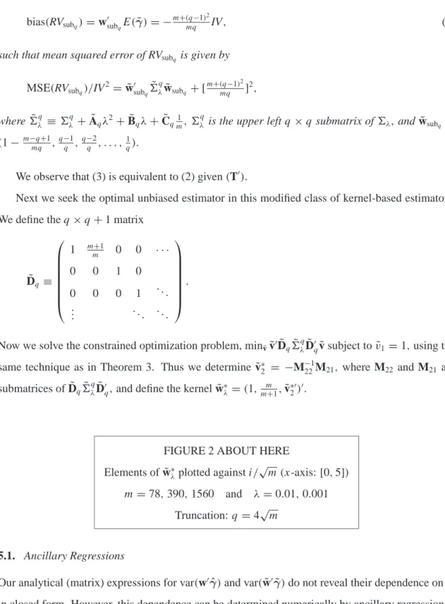
Next we seek the optimal unbiased estimator in this modified class of kernel-based estimators. We define the q×q+1 matrix
˜ Dq ≡ 1 mm+1 0 0 · · · 0 0 1 0 0 0 0 1 . .. .. . . .. ... .
Now we solve the constrained optimization problem, minv˜v˜′D˜q6˜ q
λD˜′qv subject to˜ v˜1 =1,using the same technique as in Theorem 3. Thus we determine v˜∗2 = −M22−1M21, where M22 and M21 are submatrices ofD˜q6˜
q
λD˜′q,and define the kernelw˜∗λ =(1,
m
m+1,v˜∗′2)′.
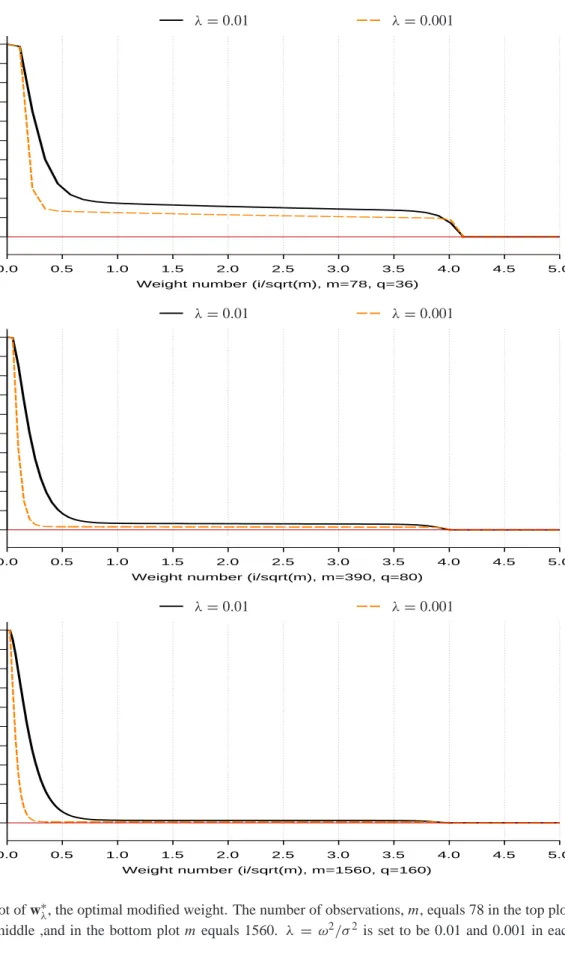
FIGURE 2 ABOUT HERE
Elements ofw˜∗λplotted against i/√m(x-axis: [0,5])
m =78,390,1560 and λ=0.01,0.001 Truncation: q =4√m
5.1. Ancillary Regressions
Our analytical (matrix) expressions for var(w′γˆ)and var(w˜′γ˜)do not reveal their dependence on m
For the regular kernel estimator we found that var(w∗′λγˆ) → 4ω4as m → ∞,and the rate at
which the variance converges to the lower bound can be determined from the ancillary regression
log(w∗′λ6λw∗λ−4λ2)=α+βlog m+εm, for m=mmin, . . . ,mmax.
Similarly for the modified kernel estimator and the subsampling estimator where log(w˜∗′λ6˜
q
λw˜∗λ)and
log(w˜′sub
q∗6˜ q
λw˜subq∗)are the relevant dependent variables. For the latter q∗ =q∗(λ,m)denotes the number of subsamples that minimized the variance.
1. Let Ymi =log(w∗′λ6λw∗λ−4λ 2),log(
˜
w∗′λ6˜λqw˜∗λ)(using truncation 4√m)or log(w˜′sub
q∗6˜ q
λw˜subq∗) (using optimal q).
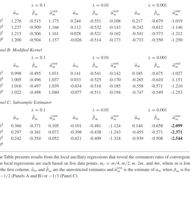
For m =103,104,105,106,run the regressions: Ymi =αm+βmlog mi+εmi, for mi = 1 4m, 1 2m,m,2m,4m, which yields(αˆm,βˆm).
2. By imposingβ= −1/2 (orβ = −1/3)reestimateαm by
ˆ αm = 1 5 5 X i=1 (Ymi −βlog mi),
TABLE 1 ABOUT HERE Ancillary Regression Results: One Panels for each of RVw∗λRVw˜∗λRVsubq∗.
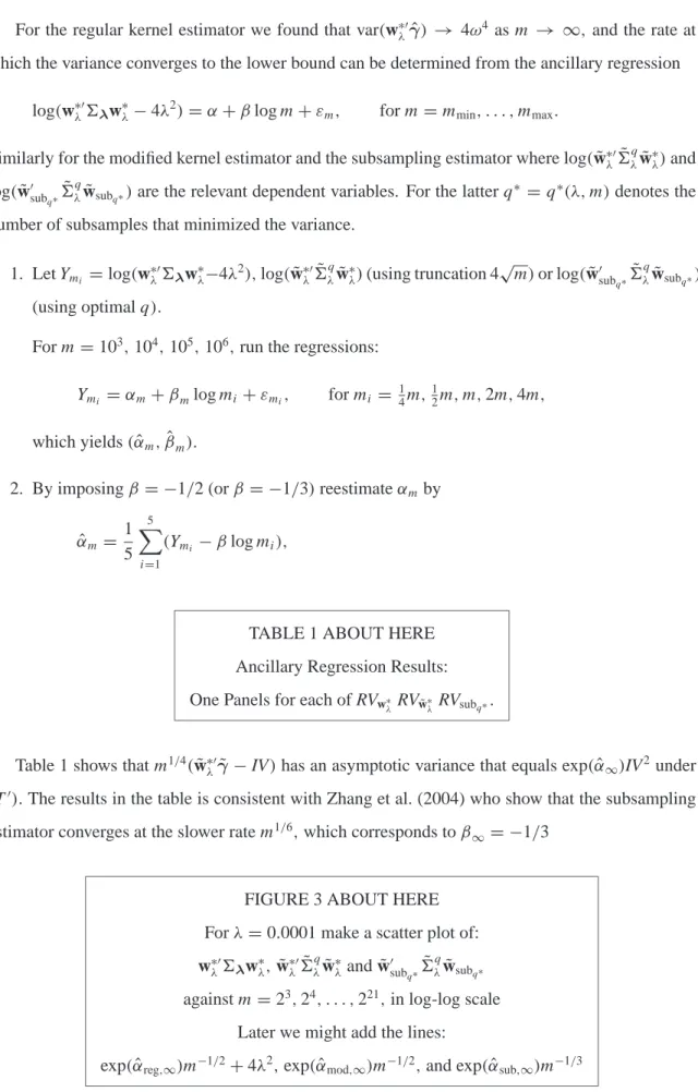
Table 1 shows that m1/4(w˜∗′
λγ˜ −IV)has an asymptotic variance that equals exp(αˆ∞)IV 2under (T′).The results in the table is consistent with Zhang et al. (2004) who show that the subsampling estimator converges at the slower rate m1/6,which corresponds toβ
∞= −1/3
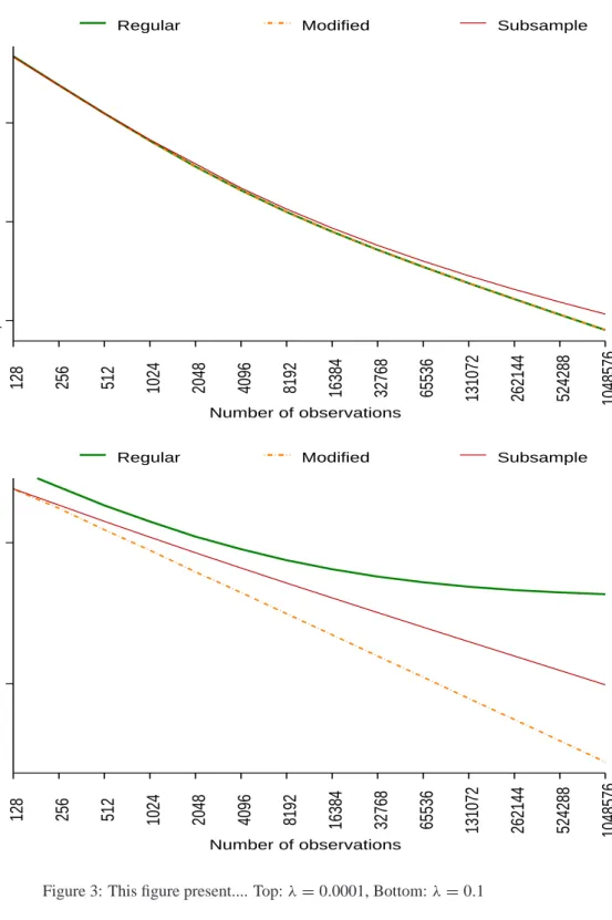
FIGURE 3 ABOUT HERE Forλ=0.0001 make a scatter plot of:
w∗′λ6λw∗λ,w˜∗′λ6˜ q
λw˜∗λandw˜′subq∗6˜
q
λw˜subq∗ against m =23,24, . . . ,221,in log-log scale
Later we might add the lines:
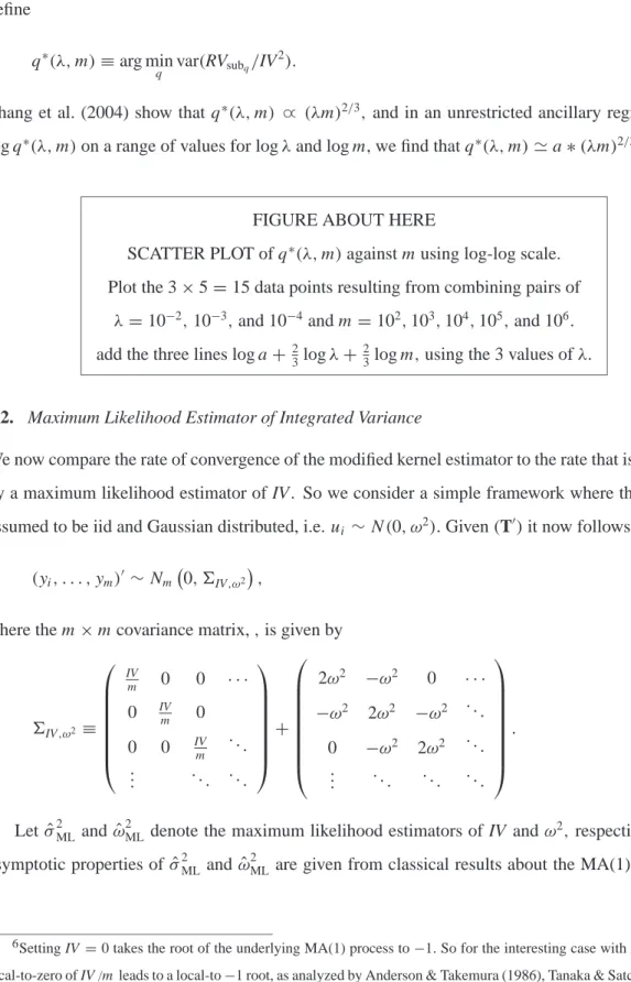
We use Theorem 8 to determine the number of subsamples that minimized the variance, and define
q∗(λ,m)≡arg min
q var(RVsubq/IV
2).
Zhang et al. (2004) show that q∗(λ,m) ∝ (λm)2/3,and in an unrestricted ancillary regression of log q∗(λ,m)on a range of values for logλand log m, we find that q∗(λ,m)≃a∗(λm)2/3.
FIGURE ABOUT HERE
SCATTER PLOT of q∗(λ,m)against m using log-log scale. Plot the 3×5=15 data points resulting from combining pairs of
λ=10−2,10−3,and 10−4and m=102,103,104,105,and 106. add the three lines log a+23logλ+ 23log m,using the 3 values ofλ.
5.2. Maximum Likelihood Estimator of Integrated Variance
We now compare the rate of convergence of the modified kernel estimator to the rate that is achieved by a maximum likelihood estimator of IV. So we consider a simple framework where the noise is assumed to be iid and Gaussian distributed, i.e. ui ∼N(0, ω2).Given(T′)it now follows that
(yi, . . . ,ym)′ ∼Nm 0, 6IV,ω2,
where the m×m covariance matrix,,is given by
6IV,ω2 ≡ IV m 0 0 · · · 0 IVm 0 0 0 IVm . .. .. . . .. ... + 2ω2 −ω2 0 · · · −ω2 2ω2 −ω2 . .. 0 −ω2 2ω2 . .. .. . . .. . .. ... .
Letσˆ2ML andωˆ2ML denote the maximum likelihood estimators of IV andω2,respectively. The asymptotic properties of σˆ2ML andωˆ2ML are given from classical results about the MA(1) process.6
6Setting IV=0 takes the root of the underlying MA(1) process to−1.So for the interesting case with IV >0,the
local-to-zero of IV /m leads to a local-to−1 root, as analyzed by Anderson & Takemura (1986), Tanaka & Satchell (1989), and Shephard (1993). However, IV /m is sufficiently “non-local” to zero that it does not affect the limiting (Gaussain) distribution of the maximum likelihood estimators.
By adopting the expression given in A¨ıt-Sahalia et al. (2003, proposition 1) to our notation, we have that asymptotic covariance matrix for(σˆ2ML,ωˆ2ML)is given by
IV2 m2 2m+4m √ 4λm+1 − 2mλ+1+√4mλ+1 • 1 2m(2mλ+1) 2mλ+1+ √ 4mλ+1 . So forλ >0 we have avar m 1/4σˆ2 ML m1/2ωˆ2ML =IV2 8 √ λ 0 0 2λ2 ,
where avar(·)denotes the asymptotic covariance matrix. This shows that the maximum likelihood estimator of IV converges at the same rate, m1/4,as the modified kernel estimator, which indeed has been show to be the optimal rate of convergence in this context, see Gloter & Jacod (2001a, 2001b). Furtherωˆ2MLconverges at the faster rate, m1/2,and since there limit distribution is Gaussian, see e.g. A¨ıt-Sahalia et al. (2003), we note that the two estimators are asymptotically independent.
The special case where there is no market microstructure noise,(λ=0)results in faster rates of convergence. Specifically we find that,
avar m 1/2σˆ2 ML m3/2ωˆ2ML =IV2 6 −2 −2 1 , and it is interesting to note that avar(m1/2σˆ2
ML)=6IV
2.So the asymptotic variance of ˆ
σ2MLis in this case three times that of the realized variance, which is the constrained(λ=0)maximum likelihood estimator. Thus the loss in estimating the nuisance parameterω2, when it is truly zero, is identical to that of RVAC(m1) ≡ ˆγ0+2γˆ1,which also has var(RVAC(m1))=6IV2 1m +o(m1)whenω2 =0,see Zhou (1996).
6. Practical Implementation
In practiceλis not known, however it is straightforward to estimateω2.Combining results of The-orem 2 concerning RV ≡ ˆγ0and our results for RVw˜ ≡ ˜w′γ˜ shows that
ˆ
ω2≡ RV−RVw˜ 2m
p
→ω2,
since E(RV) = IV +2ω2m, var(RV) = O(m)and RVw˜
p
→ IV.Given the consistency of RVw˜ it
follows that ˆ λ≡ RV−RVw˜ 2mRVw˜ = ˆ γ0− ˜w′γ˜ 2m· ˜w′γ˜ p →λ.
1. Given some initial value forλ(λosay), we constructw˜∗λo,and estimate ˆ λ= ˆλ(λo)≡max ˆ γ0− ˜w∗′λoγ˜ 2m· ˜w∗′λoγ˜ ,0 . 2. Givenλˆ we determinew˜∗ˆ
λ, and define our two-step estimator of IV to be:
RVw˜∗ ˆ λ≡ ˜w ∗′ ˆ λγ˜.
Naturally this procedure could be iterated, increasing the precision of our estimate ofλ.
What is the MSE loss of this procedure, compared to knowing the true value ofλ? [Simulation Study to be added].
7. Conclusion
We have provided a systematic analysis of regular kernel-based estimators under the assumption that market microstructure noise is independent of the efficient prices and independent of itself (at different points in time). While this assumption is reasonable when prices are not sampled too frequently, such as every 15 ticks or so, there is overwhelming evidence that market microstructure noise has a more sophisticated dependence structure when sampling occurs at ultra-high frequencies, such as every tick. We are therefore, in separate papers, extending our analysis of kernel-based estimators to the situation with more general assumptions about the noise process.
We have showed that regular kernel-based estimators can be quite accurate estimators of quadratic variation, however they are always inconsistent. Taking inspiration from the consistent subsampling estimator, a new modified kernel estimator is suggested which is consistent and has good finite sample properties.
A. Proof of Theorem 2 and Related Results
Proof of Lemma 1. First we note that t⌈sm⌉−1,m =t⌈(s−1
m)m⌉,m and by(T)we have that sup s∈[0,1] (t⌈sm⌉,m−t⌈sm⌉−1,m)−(τ (s)−τ (s−m1)) =o(m−1), such that sup s∈[0,1] t⌈sm⌉,m−t⌈sm⌉−1,m 1/m −τ ′(s) ≤ sup s∈[0,1] t⌈sm⌉,m−t⌈sm⌉−1,m 1/m − τ (s)−τ (s−m1) 1/m + sup s∈[0,1] τ′(s)− τ (s)−τ (s− 1 m) 1/m =o(1)+o(1), (A.1)
where the last term is o(1)sinceτ′is bounded. (A.1) clearly implies the result stated in the Lemma, (the two are equivalent given the continuity ofτ′(s)).
Lemma A.1 We define xi,h≡ yiyi+h.Given(N)and(V)we have that
Part I E(xi,h) var(xi,h) cov(xi,h,xi±1,h) h=0 σ2i +2ω2 (2κ+2)ω4+8ω2σ2i +2σ4i (κ−1)ω4
h=1 −ω2 (κ+2)ω4+2ω2(σi2+σ2i+1)+σ2iσ2i+1 ω4
h ≥2 0 4ω4+2ω2(σ2i +σ2i+h)+σi2σ2i+h ω4
while cov(xi,h,xi±k,h)=0, k≥2 for all h =0,1, . . . .
Part II cov(xi,h,xi,h+1) cov(xi,h,xi−1,h+1) cov(xi,h,xi−1,h+2)
h=0 −(κ +1)ω4−2ω2σ2i −(κ+1)ω4−2ω2σ2i 2ω4
h ≥1 −2ω4−ω2σ2i −2ω4−ω2σ2i+h ω4,
while all other covariance terms are zero.
Proof. (Part I) The expected values are given from
E(xi,h)= E(yiyi+h)= E(yi∗+ui −ui−1)(yi∗+h+ui+h−ui+h−1),
which shows that E(xi,0)= E(yi∗2)+E(ui)2+E(u2i−1)=σ2i+2ω2,since yi∗,ui,and ui−1are pair-wise uncorrelated. Similarly we find that E(xi,1)= E [(ui)(−ui)]+0= −ω2and that E(xi,h)=0 for h ≥2.
Next, we turn to the variance and covariance terms, where we make use of the identities, var(ei)=E(e2i)=2ω2and E(ei4)=E [u4i +u4i−1+6u2iu2i−1−4uiui3−1−4u3iui−1]=(2κ+6)ω4. For h =0 we have E(xi2,0)= E(yi4)= E(yi∗+ei)4=E(yi∗4)+E(e 4 i)+6E(y∗ 2 i e 2 i)=3σ 4 i +(2κ+6)ω 4 +6σ2i2ω2, and E(xi,0xi+1,0) = E(yi2y 2 i+1)=E(yi∗+ei)2(yi∗+1+ei+1)2 = E [(yi∗2+ei2+2yi∗ei)(yi∗+21+e 2 i+1+2yi∗+1ei+1)] = E [(yi∗2+ei2)(yi∗+21+ei2+1)]=E [(yi∗2+u2i +u2i−1)(yi∗+21+u2i+1+u2i)]
= σ2iσ2i+1+(σ2i +σ2i+1)2ω2+(κ+3)ω4, (A.2) E(xi,0xi+h,0) = E(yi2y 2 i+h)=σ 2 iσ 2 i+h+(σ 2 i +σ 2 i+h)2ω 2 +4ω4, for h≥2, (A.3) such that var(xi,0) = E(xi2,0)−[E(xi,0)]2=[3σ4i +(2κ+6)ω 4 +12σ2iω2]−[σ2i +2ω2]2 = 2σ4i +(2κ+2)ω4+8σ2iω2,
cov(xi,0,xi+1,0) = (κ−1)ω4, and cov(xi,0,xi+h,0)=0 for h ≥2. For h =1 we find E(xi2,1)= E(yi2yi2+1)= E(xi,0xi+1,0)which is derived in (A.2),
E(xi,1xi+1,1) = E(yi∗+ui −ui−1)(yi∗+1+ui+1−ui)2(yi∗+2+ui+2−ui+1) = E [(ui)(−2ui+1ui)(−ui+1)]=2E [uiui+1uiui+1]=2ω4,
and E(xi,1xi+2,1)=ω4.Since E(xi,1)E(xj,1)=(−ω2)(−ω2)=ω4for all i,j =1, . . . ,m,we find that var(xi,1) = σ2iσ 2 i+1+(σ 2 i +σ 2 i+1)2ω 2 +(κ+3)ω4−(ω2)2 = σ2iσ2i+1+(σ2i +σi2+1)2ω2+(κ+2)ω4,
and cov(xi,1,xi+1,1)=ω4and cov(xi,1,xi+h,1)=0,for h ≥2.
For h ≥ 2 we have E(xi2,h) = E(yi2yi2+h) = E(xi,0xi+h,0)which is derived in (A.3), such that var(xi,h)=σ2iσ2i+h+2(σ2i +σ2i+h)ω2+4ω4.Next, we have that
E(xi,hxi+1,h)=E(eiei+hei+1ei+1+h)=ω4,
while E(xi,hxi+k,h)=0 for k≥2.So cov(xi,h,xi±1,h)=ω4and cov(xi,h,xi±k,h)=0 for k ≥2.
(Part II) We consider
E(xi,0xi,1) = E(yi2yiyi+1)= E [(yi∗+ei)3(yi∗+1+ei+1)] = E [(yi∗2+2yi∗ei+e2i)(yi∗+ei)(−ui)] = E [(yi∗2+2yi∗ei+e2i)(yi∗+ui−ui−1)(−ui)] = −σ2iω2−2σ2iω2+E [ei2(ui −ui−1)(−ui)] = −σ2iω2−2σi2ω2+E [(u2i +u 2 i−1−2ui−1ui)(ui −ui−1)(−ui)] = −σ2iω2−2σ2iω2−κω4−ω4−2ω4= −3σ2iω2−(κ+3)ω4, such that cov(xi,0,xi,1)= −3σ2iω
2
−6ω4−(σ2i+2ω2)(−ω2)= −2σ2iω2−(κ+1)ω4,and similarly E(xi,0xi−1,1) = E(yi2yi−1yi)=E [(yi∗2+2yi∗ei+e2i)(yi∗+ui−ui−1)(ui−1)]
= −σ2iω2−2σ2iω2+E [ei2(ui −ui−1)(ui−1)]
= −σ2iω2−2σ2iω2+E [(ui2+u2i−1−2ui−1ui)(ui −ui−1)(ui−1)] = −σ2iω2−2σ2iω2−ω4−κω4−2ω4= −3σ2iω2−(κ+3)ω4, which shows that cov(xi,0,xi−1,1)= −2σ2iω
2 −(κ+1)ω4.For k≥1 we have E(xi,0xi+k,1) = E [(yi∗2+2yi∗ei+ei2)(yi∗+k+ei+k)(yi∗+k+1+ei+k+1)] = E [(yi∗2+2yi∗ei+e2i)(−u 2 i+k)] = −E [(yi∗2+u2i +u2i−1)(u2i+k)]= −σ2iω2−2ω4, and similarly for k ≤ −2.Thus cov(xi,0,xi+k,1)=0 for k ≥1 and k ≤ −2.
The only non-zero covariance between xi,0and xi+k,2,is
cov(xi,0,xi−1,2)=cov(e2i,ei−1ei+1)=E(e2iui−1(−ui))=E(2u2i−1u 2
i)=2ω
4 ,
and for j ≥3 we find that cov(xi,0,xi+k,j)=0 for all k. For h≥1 we have cov(xi,h,xi,h+1) = E(yiyi+hyiyi+h+1)= E [yi2ui+h(−ui+h)]= −(σi2+2ω 2)ω2, cov(xi,h,xi−1,h+1) = E(yiyi+hyi−1yi+h)= E [−ui−1ui−1yi2+h]= −(σ 2 i+h+2ω 2)ω2,
and similarly cov(xi,h,xi−1,h+2)=E(eiei+hei−1ei+h+1)= E(−ui−1)(ui+h)(ui−1)(−ui+h)=ω4.
Lemma A.2 (a)Pmi=−1h(σ2i +σ2i+h) =2R01ψh m(s)σ
2(s)ds, and(b)given(V)and q
m = O(m1/2) it holds that m mX−qm i=1 σ2iσ2i+q m − Z 1 0 ψqm m (s)σ 4 (s)ds=o(1). Proof.(a)Sinceσ2i =R i m i−1 m
σ2(s)ds, the first result follows from the identityPmi=−1hσi2=R m−h m 0 σ 2(s)ds. (b)We note thatPm−qm i=1 σ 2 iσ 2 i+qm = Pm−qm i=1 [σ 4 i+σ 2 i(σ 2 i+qm−σ 2
i)] and similarly that Pm−qm i=1 σ 2 iσ 2 i+qm = Pm−qm i=1 [σ 4 i+qm −σ 2 i+qm(σ 2 i+qm −σ 2 i)] such that mX−qm i=1 σ2i,mσ2i+q m,m = 1 2 mX−qm i=1 (σ4i,m+σ4i+q m,m)− 1 2 mX−qm i=1 (σ2i+q m,m−σ 2 i,m) 2 . (A.4)
First we consider the first term on the right hand side. Letδi,m ≡ti,m−ti−1,m and note thatδi,m = O(m−1) given(T). So for arbitrary pairs (si,m,s˜i,m),i = 1, . . . ,m of points, where si,m,s˜i,m,∈
[ti−1,m,ti,m] we have that
m mX−qm i=1 |σ4(si,m)−σ4(s˜i,m)|δ2i,m = m− 1/2 mX−qm i=1 |σ4(si,m)−σ4(s˜i,m)|δ2i,mm 3/2