Flexible semiparametric mixed models

Tutz, Reithinger:

Flexible semiparametric mixed models

Sonderforschungsbereich 386, Paper 448 (2005)

Online unter: http://epub.ub.uni-muenchen.de/

Flexible Semiparametric Mixed Models

Gerhard Tutz & Florian Reithinger

Ludwig-Maximilians-Universit¨at M¨unchen Akademiestraße 1, 80799 M¨unchen

{tutz,flo}@stat.uni-muenchen.de

27.07.2005

Abstract

In linear mixed models the influence of covariates is restricted to a strictly parametric form. With the rise of semi- and nonparametric regression also the mixed model has been expanded to allow for additive predictors. The common approach uses the representation of additive models as mixed models. An alternative approach that is proposed in the present paper is likelihood based boosting. Boosting originates in the machine learning community where it has been pro-posed as a technique to improve classification procedures by combining estimates with reweighted observations. Likelihood based boosting is a general method which may be seen as an extension of L2 boost. In additive mixed models the advantage of boosting techniques in the form of componentwise boosting is that it is suitable for high dimensional settings where many influence variables are present. It allows to fit additive models for many covariates with implicit selection of relevant variables and automatic selection of smoothing parameters. Moreover, boosting tech-niques may be used to incorporate the subject-specific variation of smooth influence functions by specifying ”random slopes” on smooth effects. This results in flexible semiparametric mixed models which are appropriate in cases where a simple random intercept is unable to capture the variation of effects across subjects.

Keywords: Mixed Model, boosting, random slopes, additive models, smoothing

1

Introduction

There is an extensive body of literature on the linear mixed model, early highlights being Hen-derson (1953), Laird & Ware (1982) and Harville (1977). Nice overviews including more recent work are found in Verbeke & Molenberghs (2001), McCulloch & Searle (2001). In common linear mixed models the influence of covariates is restricted to a strictly parametric form. While in regression models much work has been done to extend the strict parametric form to more flexible forms of semi- and nonparametric regression, much less has been done to develop flexible mixed model. For overviews on semiparametric regression models see Hastie & Tibshirani (1990), Green & Silverman (1994) and Schimek (2000).

A first step to more flexible mixed models is the generalization to additive mixed models where a random intercept is included. With responseyit for observation t on individual i and

covariatesui1, . . . uim the basic form is

where α(1)(.), . . . , α(m)(.) are unspecified functions of covariates ui1, . . . , uim, bi0 is a

subject-specific random intercept withbi0∼N(0, σb2) andεitis an additional noise variable. Estimation

for this model may be based on the observation that regression models with smooth compo-nents may be fitted by mixed model methodology. Speed (1991) indicated that the fitted cubic smoothing splines is a best linear unbiased predictor. Subsequently the approach has been used in several papers to fit mixed models, see e.g. Verbyla, Cullis, Kenward & Welham (1999), Parise, Wand, Ruppert & Ryan (2001), Lin & Zhang (1999), Brumback & Rice (1998), Zhang, Lin, Raz & Sowers (1998),Wand (2003). Bayesian approaches have been considered e.g. by Fahrmeir & Lang (2001).

In model (1) it is assumed that the effects of covariates do not vary across individuals. This restriction is rather severe. For example in the analysis of growth curves it has to be assumed that not only the starting values differ for individuals but also that the speed of growth depends on individuals. In order to avoid overparameterization we propose to model the variation across individuals by random ”slopes” of smooth functions. A simple model of this type is

yit=βo+α(ui) +bi0+bi1α(ui) +εit, (2)

where for simplicity only one variableui is considered which has the smooth effect α(ui) but

which is modified by the random effect bi1. By assuming (bi0, bit)∼N(0,Σb) the intercept as

well as the slope are considered as subject-specific random effects. Model (2) raises problems in estimation since the random slopesbi1are linked to the functionα(ui) which is not a known

pre-dictor as in the usual linear mixed model. In order to illustrate flexible models we will consider the following examples.

Application 1: AIDS Study

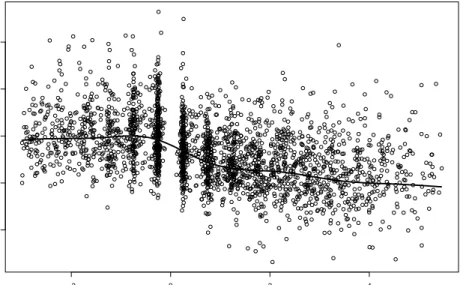
The data were collected within the Multicenter AIDS Cohort Study (MACS), which has fol-lowed nearly 5000 gay or bisexual men from Baltimore, Pittsburgh, Chicago and Los Angeles since 1984 (see Kaslow, Ostrow, Detels, Phair, Polk & Rinaldo (1987), Zeger & Diggle (1994)). The study includes 1809 men who were infected with HIV when the study began and another 371 men who were seronegative at entry and seroconverted during the follow-up. In the study 369 seroconverters with 2376 measurements in total were used, two subjects were dropped since covariate information was not available. The interesting response variable is the number or per-cent of CD4 cells by which progression of disease may be assessed. Covariates include years since seroconversion, packs of cigarettes a day, recreational drug use (yes/no), number of sexual partners, age and a mental illness score. Zeger & Diggle (1994) motivate extensively the interest in the typical time course of CD4 cell decay and the variability across subjects. Since the forms of the effects is not known, time since seroconversion, age and the mental illness score may be considered as unspecified additive effects. Figure 1 shows the smooth effect of time on CD4 cell decay for a random intercept model together with the data, Figure 2 shows the observations for three men with differing number of observed time points (dashed lines) and the fitted curves for individual time decay (for details see Section 3).

Application 2: Jimma Study

The Jimma Infant Survival Differential Longitudinal Study which is extensively described in Lesaffre, Asefa & Verbeke (1999) is a cohort study examining the live births which took place during a one year period from September 1992 until September 1993 in Ethiopia. The study involves about 8000 households with live births in that period. The children were followed up for one year to determine the risk factors for infant mortality. Following Lesaffre, Asefa & Verbeke (1999) we consider 495 singleton live births from the town of Jimma and look for the determinants of growth of the children in terms of body weight (in kg). Weight has been measured at delivery and repeatedly afterwards. In addition we consider the socio-economic and demographic covariates age of mother in years (AGEM), educational level of mother (0-5: illiterate, read and write, elementary school, junior high school, high school, college and above), place of delivery (DELIV,1-3: hospital, health center, home), number of antenatal visits (VISIT,

−2 0 2 4 10 20 30 40 50 time sqrtcd4

Figure 1: Smoothed time effect on the CD4 cell from Multicenter AIDS Cohort Study (MACS)

−2 −1 0 1 2 3 4 15 20 25 30 35 40 45 1 2

Figure 2: Smoothed time effect on the CD4 cell from Multicenter AIDS Cohort Study (MACS) and the decay of CD4 cells of 3 members of the study over time

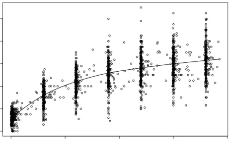
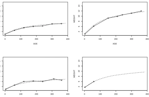
0,>1), month of birth (TIME,1:Jan.-June, 0:July-Dec.), sex of child (1:male, 0:female). For more details and motivation of the study see Lesaffre, Asefa & Verbeke (1999). Figure 3 shows the overall evolution of weight and Figure 4 shows the growth curve of four children (observations and fitted curves) for an additive mixed model with random slopes on the additive age effect. It is seen that random slopes are definitely necessary for modelling since speed of growth varies strongly across children.

In the following estimation procedures are proposed for the additive model as well as for models with random slopes on smooth effects. In the case of the additive model they may be seen as an alternative to the approach based on Speed’s (1991) observation. To our knowledge the fitting of random slopes of smooth effects has not been considered in the literature because of the underlying multiplicative structure of effects. The proposed estimation procedures for both semiparametric structures are based on boosting techniques which for regression models have been suggested e.g. by B¨uhlmann & Yu (2003). It is shown that in particular in high dimensional settings boosting approaches yield quite efficient estimation procedures for additive models and they may be modified to allow random slopes of curves.

In Section 2 the additive mixed model is considered. It is shown how estimates of parameters and variances are obtained for given smoothing parameters and how smoothing parameters may be obtained as ML or REML estimates. In Section 3 the proposed estimators are outlined. By utilizing boosting techniques the selection of potentially high dimensional smoothing parameters is avoided and stable estimates are obtained. It is shown that in particular in high dimensional problems where many unspecified procedures of potential influence have to be considered the boosting approach outperforms alternative approaches. Moreover, the CD4 cells example is considered in section 3. In Section 4 the modelling of random slopes of smooth effects is considered and an estimation technique is given that is able to cope with the multiplicative structure of effects. In Section 5 extensions to varying-coefficients models and interactions is briefly sketched.

0 100 200 300 400 2 4 6 8 10 12 AGE WEIGHT

0 100 200 300 400 4 6 8 10 12 14 AGE WEIGHT 0 100 200 300 400 4 6 8 10 12 14 AGE WEIGHT 0 100 200 300 400 4 6 8 10 12 14 AGE WEIGHT 0 100 200 300 400 4 6 8 10 12 14 AGE WEIGHT

Figure 4: Individual infant curves (observed and predicted)

2

Additive Mixed Model

2.1

The Model

Let the data be given by (yit, xit, uit, wit), i= 1, . . . , n, t= 1, . . . , Ti, whereyitis the response

for observation t within cluster i and xT

it = (xit1, . . . , xitp), uTit = (uit1, . . . , uitm), wTit =

(wit1, . . . , wits) are vectors of covariates, which may vary across clusters and observations. The

semiparametric mixed model that is considered in the following has the general form yit=xTitβ+ m X j=1 α(j)(uitj) +witTbi+ǫit =µpar_it +µadd it +µrandit +ǫit (3) where

µparit =xTitβ is a linear parametric term,

µadd

it =

Pm

j=1α(j)(uitj) is an additive term with unspecified influence functionsα(1), . . . , α(m),

µrand

it =witTbicontains the cluster-specific random effectbi, bi∼N(0, Q(ρ)), whereQ(ρ) is a

parameterized covariance matrix and

ǫit is the noise variable,ǫit∼N(0, σ2I), ǫit, bi independent.

In spline methodology the unknown functionsα(j)are approximated by basis functions. A simple

basis is known as the truncated power series basis of degreed, yielding α(j)(u) =γ0(j)+γ (j) 1 u+. . . γ (j) d u d₊ M X s=1 α(sj)(u−ks(j))d+, wherek(1j)< . . . < k (j)

M are distinct knots. More generally one uses

α(j)(u) = M X

s=1

where Φ(sj) denotes the s-th basis function for variable j, αTj = (α

(j)

1 , . . . , α

(j)

M) are unknown

parameters and Φj(u)T = (Φ(1j)(u), . . . ,Φ

(j)

M(u)) represent the vector-valued evaluations of the

basis functions.

For semi- and nonparametric regression models Eilers & Marx (1996), Marx & Eilers (1998) propose the numerically stable B-splines which have also been used by Wood (2004). For further investigation of basis functions see also Wand (2000), Ruppert & Carroll (1999).

By collecting observations within one cluster the model has the form yi = Ziβ+ Φi1α1+. . .+ Φimαm+Wibi+ǫi, ǫi bi ∼N 0 0 , σ2 εI Q(ρ) , (5)

whereZiβ contains the linear term, Φijαj represents the one additive term andWiβ the random

term. Vectors and matrices are given by yT

i = (yi1, . . . , yiTi), ZiT = (xi1, . . . , xiTi),ΦTij =

(Φ(1j)(ui1j), . . . ,Φ(Mj)(uiTij)), WiT = (wi1, . . . , wiTi), ǫTi = (ǫi1, . . . , ǫiTi). In the case of the

truncated power series the ”fixed” termγ₀(j)+γ₁(j)u+. . .+γ(_dj)ud _{is taken into the linear term}

Ziβ without specifyingZi andβ explicitly.

In matrix form one obtains

y=Zβ+ Φ1α1+. . .+ Φmαm+W b+ǫ

whereyT _{= (y}T

1, . . . , yTn), bT = (bT1, . . . , bTn), ǫT = (ǫT1, . . . , ǫTn),

ZT _{= (Z}T

1, . . . , ZnT), ΦTj = (ΦT1j, . . . ,ΦTnj), WT = (W1T, . . . , WnT).

Parameters to be estimated are the fixed effects, collected in δT _{= (β}T_{, α}T

1, . . . , αTm) and the

variance specific parametersθT _{= (σ}

ε, ρT) which determine the covariancescov(ǫit) =σ2εITi and

cov(bi) =Q(ρ). In addition one wants to estimate the random effects bi. Since bi is a random

variable the latter is often called prediction rather than estimation.

2.2

Penalized Maximum Likelihood Approach

Starting from the marginal version of the model

yi=Ziβ+ Φi1α1+. . .+ Φimαm+ǫ∗i, (6)

ǫ∗

i ∼N(0, Vi(θ)), Vi(θ) =σ2ITi+WiQ(ρ)WiT,

estimates forδmay be based on thepenalized log-likelihood

lp(δ;θ) =−1 2 n X i=1 log(|Vi(θ)|)− n X i=1 1 2(yi−Ziδ) T_(V i(θ))−1(y−Ziδ)−1 2δ T_{Kδ, (7)}

where δT_{Kδ is a penalty term which penalized the coefficients α}

1, . . . , αn. For the truncated

power series an appropriate penalty is given by

K=Diag(0, λ1I, . . . , λmI),

where I denotes the identity matrix and λj steers the smoothness of the function α(j). For

λj → ∞ a polynomial of degreed is fitted. P-splines ((Eilers & Marx 1996)) use K = DTD

whereD is a matrix that builds the difference between adjacent parameters yielding the penalty δT_{Kδ= Σ}

jλjΣs(α(sj+1) −α

(j)

s )2or higher differences.

From the derivative of lp(δ, θ) one obtains the estimation equation ∂lp(δ, φ)/∂δ = 0 which

yields n X i=1 (ZiT(Vi(θ))−1yi) = ( n X i=1 (ZiT(Vi(θ))−1Zi+K)−1)ˆδ

and therefore ˆ δ= ( n X i=1 (ZiT(Vi(θ))−1Zi+K))−1 n X i=1 ZiT(Vi(θ))−1yi

which depends on the variance parametersθ. It is well known that maximization of the log-likelihood with respect to θ yields biased estimates since maximum likelihood does not take into account that fixed parameters have been estimated (see Patterson & Thompson (1974)). The same holds for the penalized log-likelihood (7). Therefore for the estimation of variance parameters often restricted maximum likelihood estimates (REML) are preferred which are based on the log-likelihood lr(δ, θ) = −1 2 n X i=1 log(|Vi(θ)|)−1 2 n X i=1 (yi−Ziβ)TVi(θ)−1(yi−Ziβ) −1 2 n X i=1 log(|ZiTVi(θ)Zi|),

see Harville (1974), Harville (1977) and Verbeke & Molenberghs (2001).

The restricted log-likelihood differs from the log-likelihood by an additional component. One has lr(δ, θ) =l(δ, θ)− 1 2 n X i=1 log(|ZiTVi(θ)Zi|).

It should be noted that for the estimation ofθthe penalization termδT_{Kδmay be omitted since}

it has no effect. Details on REML is given in the Appendix.

BLUP Estimates

Usually one also wants estimates of the random effects. Best linear unbiased prediction (BLUP) is a framework to obtain estimates forβ andb1, . . . , bnfor given variance components. There are

several ways to motivate BLUP (see Robinson (1991)). One way is to consider the joint density ofy andb which is normal and maximize with respect toδ andb. By adding the penalty term δT_{Kδ one has to minimize}

n X i=1 1 σ2(yi−ZΦiδ−Wibi) T_(y i−ZΦiδ−Wibi) +bTiQ(ρ) −1_b i+δTKδ (8) whereZΦi= [Zi,Φi1, . . . ,Φim], ¯Q(ρ) =Diag(Q(ρ). . . Q(ρ)). WithZT

Φ = (ZΦ1T . . . ZΦTm) the criterion (8) may be rewritten as

1

σ2(y−ZΦδ−W b)

T_(y−Z

Φδ−W b) +bTQ(ρ)¯ −1bT +δTKδ

which yields the ”ridge regression” solution

ˆ δ ˆ_b =CT 1 σ2 εIC+B −1 CT 1 σ2 ε Iy withC= (ZΦ, W) and B= K 0 0 Q(ρ)¯ −1 . Some matrix derivation shows that ˆδhas the form

ˆ

δ= (ZΦTV(θ)

−1_Z

whereV(θ) =Diag(V1(θ). . . Vn(θ)), and for the vector of random coefficientsbT = (bT1, . . . , bTn)

one obtains

ˆ_b=Q(ρ)WT_V(θ)−1_(y−Z

Φδ).ˆ

In simpler form BLUP estimates are given by ˆ δ= ( n X i=1 (ZiT(Vi(θ))−1Zi+K))−1 n X i=1 ZiT(Vi(θ))−1yi, ˆ_bi=QWT i Vi(θ)−1(yi−ZΦiδ).ˆ

2.3

Mixed Model approach to Smoothing

For the computation of ˆδ it is necessary to specify the smoothing parametersλ1, . . . , λm. With

cross-validation techniques problems arise if the number of smooth covariates is high. An ap-proach that works for moderate number of smooth covariates uses the ML or REML estimates of variance components. The basic concept ist to reformulate the estimation as a more general mixed model. Let us consider again the criterion for BLUP estimates (8) which has the form

1 σ2(y−ZΦδ−W b) T_(y−Z Φδ−W b) +αTKαα+bTQ(ρ)¯ −1b = 1 σ2(y−Zβ−Φα−W b) T_{(y−Zβ−Φα−W b) + (α}T_bT₎ Kα 0 0 Q(ρ)¯ −1 α b (9) where Φ = [Φ1. . .Φm] andKαfor the truncated power series has the formKα=Diag(λ1I, . . . , λmI).

Thus (9) corresponds to the BLUP criterion of the mixed model y=Zβ+ Φ W α b +ǫ with   α b ǫ  ∼N     0 0 0  ,   K−1 α 0 0 0 Q(ρ)¯ 0 0 0 σ2 εI    .

Since Kα = Diag(λ1I, . . . , λmI) the smoothing parameters λ1, . . . , λm correspond to the

vari-ance of the random effectsα1, . . . , αmfor whichcov(αj) =λjIis assumed. Thus for the purpose

of estimationα1, . . . , αmare treated as random effects. REML estimates yield ˆλ1, . . . ,ˆλm. For

alternative basis function like B-splines some reformation is necessary to obtain the simple inde-pendence structure of the random effects (see Appendix).

3

Boosting Approach to Additive Mixed

Models

Boosting originates in the machine learning community where it has been proposed as a technique to improve classification procedures by combining estimates with reweighted observations. Since it has been shown that reweighting corresponds to minimizing iteratively a loss function (Breiman (1999), Friedman (2001)) boosting has been extended to regression problems in aL2-estimation

framework by B¨uhlmann & Yu (2003).In the following boosting is used to obtain estimates for the semiparametric mixed model. Instead of using REML estimates for the choice of smoothing parameters the estimates of the smooth components are obtained by using ”weak learners” iteratively. The weak learner that is used is the estimate of δ based on a fixed, very large smoothing parameter λ which is used for all components. By iterative fitting of the residual and selection of components (see algorithm) the procedure adapts automatically to the possibly varying smoothness of components.

3.1

The boosting algorithm

The following algorithm uses componentwise boosting. Componentwise boosting means that only one component of the predictor, in our case one smooth term Φijαj, is refitted at a time.

That means that a model containing the linear term and only one smooth component is fitted in one iteration step. For simplicity we will use the notation

Zi(r)= [Zi Φir] , δTr = (βT, αTr)

for the design matrix with predictorZi(r)=Ziβ+ Φirαr.

The corresponding penalty matrix is denoted byKr, which for the truncated power series has

the form

Kr=Diag(0, λI).

BoostMixed

1. Initialization

Compute starting values ˆβ(0)_,αˆ(0) 1 , . . .αˆ

(0)

m and setηi(0)=Ziβˆ(0)+ Φi1αˆ1(0)+. . .+ Φimαˆ(0)m.

2. Iteration For l=1,2,. . .

(a) Refitting of residuals

i. Computation of parameters

Forr∈ {1, . . . , m} the model for residuals yi−η(l −1) i ∼N(ηi(r), Vi(θ)) with ηi(r)=Zi(r)δr=Ziβ+ Φirαr is fitted, yielding ˆ δr= ( n X i=1 (ZT i(r)(Vi(θ(l−1)))−1Zi(r)+Kr))−1 n X i=1 ZT i(r)(Vi(θ(l−1)))−1(yi−η(l −1) i ).

ii. Selection step

Select fromr∈ {1, . . . , m} the componentj that leads to the smallestAICr(l)or

BICr(l)as given in Section 3.2.

iii. Update Set βˆ(l)= ˆβ(l−1) + ˆβ, and ˆ α(rl)= ( ˆ α(l−1) r ifr6=j ˆ α(l−1) r + ˆαr ifr=j, ˆ δ(l)= (( ˆβ(l))T, (ˆα1(l))T, . . .(ˆα(ml))T)T. Update fori= 1, . . . , n η_i(l)=η(l−1) i +Zi(j)δˆj.

(b) Computation of Variance Components

The computation is based on the penalized log-likelihood

lp(θ|η(l);δl) =−1₂Pn_i=1log(|Vi(θ)|) +Pn_i=1(yi−η(l))TVi(θ)−1(yi−η(l))

−1

2(ˆδ

(l)₎T_Kδˆ(l)_.

We chose componentwise boosting techniques since they turn out to be very stable in the high dimensional case where many potential predictors are under consideration. In this case the procedure automatically selects the relevant variables and may be seen as a tool for variable selection with respect to unspecified smooth functions. In the case of few predictors one may also use boosting techniques without the selection step by refitting the residuals for the full model with design matrix [ZiΦi1. . .Φim].

3.2

Stopping criteria and Selection in BoostMixed

In boosting often cross-validation is used to find the appropriate complexity of the fitted model (e.g. Dettling & B¨uhlmann (2003), ...). In the present setting cross-validation turns out to be too time consuming to be recommended. An alternative is to use the effective degrees of freedom which are given by the trace of the hat matrix (compare Hastie & Tibshirani (1990)). In the following the hat matrix is derived.

For the derivation of the hat matrix the matrix representation of the mixed model is preferred (see (6))

y=Zβ+ Φ1α1+. . .+ Φmαm+ǫ∗

where ǫ∗

∼N(0, V), V(θ) =Diag(V1(θ), . . . , Vn(θ)).

Since in one step only one component is refitted one has to consider the model for the residual refit of therth component.

residual=Zrδr

where ZrT = (Z1(Tr). . . Z T

n(r)), Zi(r)= [Zi Φir], δTr = (βT, αTr).

The refit in thelth step is given by ˆ δr = ZrTV(θ(l −1) )−1 Zr+λKr −1 ZrTV −1 (θ(l−1) )(y−η(l−1) ) (10) = Mr(l)(y−η(l −1)₎ where Mr(l)= ZrTV(θ(l −1) )−1 Zr+λKr −1 ZrTV −1 (θ(l−1) )

refers to therth component in thelth refitting step. Then the corresponding fit has the form ˆ η(rl)=Zrˆδr=ZrMr(l)(y−ηˆ(l −1)_{) =H}(l) r (y−η(l −1)₎ where Hr(l)=ZrMr(l).

Let nowjldenote the index of the variable that is selected in thelth boosting step andH(l)=Hje(l)

denote the resulting ”hat” matrix of the refit. One obtains with starting matrixH(0)

η(1)=H(0)y+H(1)(y−ηˆ(0)) = (H(0)+H(1)(I−M(0)))y and more general

ˆ η(l)_=G(l)_y where G(l)= l X s=0 H(s) s−1 Y k=0 (I−H(k))

is the global hat matrix after thelth step. It is sometimes useful to rewriteGas G(l)_=I−

l Y

k=0

(compare B¨uhlmann & Yu (2003)).

For the selection step one evaluates the hat matrices for candidates which for therth component in thelth step have the form

G(rl)=G(l −1)_+H(l) r l−1 Y k=0 (I−H(k)).

Given the hat matrixG(rl), complexity of the model may be determined by information criteria.

When considering in thelth step the rth component one uses the criteria AICr(l) = −2 ( −1 2 n X i=1 log(V(ˆθ(l−1) )) + n X i=1 (yi−ηˆ(l−1))TVi(ˆθ(l−1))−1(yi−ηˆ(l−1)) ) + 2trace(G(rl)), BICr(l) = −2 ( −1 2 n X i=1 log(V(ˆθ(l−1) )) + n X i=1 (yi−ηˆ(l −1) i )(Vk(θ)(l−1))−1(yi−η(l −1) i ) ) + 2trace G(rl)log(n)

In the rth step one selects from r ∈ {1, . . . , m} the component that minimizes AICr(l)(or

BICr(l)) and obtains AIC(l) =AIC_jl(l) if jl is selected in the rth step. IfAICr(l)(or BICr(l)) is

larger than the previous criterionAIC(l−1) _{iteration stops. It should be noted that in contrast}

to common boosting procedures the selection step reflects the complexity of the refitted model. In common componentwise boosting procedures (e.g. B¨uhlmann & Yu (2003)) one selects the component that maximally improves the fit and then evaluates if the fit including complexity of the model deteriorates. The proposed procedure selects the component in a way that the new lack-of-fit, including the augmented complexity, is minimized. In our simulations the suggested approach showed superior performance.

In the following the initialization of the boosting algorithm is shortly sketched. The basic concept is to select few relevant variables in order to obtain stable estimates of variance compo-nents. Therefore for largeλ(in our appllicationλ= 1000), the total model is fitted using the full design matrix ˜Z = [Z,Φ1, . . . ,Φm] and covariance matrixVi(θ) =I. Then in a stepwise way the

variables are selected (usually up to 5) that yield the best fit. These yield the initial estimates ˆ

β(0)_{, α}(0) 1 , . . . , α

(0)

m and the initial hat matrixG(0).

3.3

Standard Errors

Approximate standard errors for the parameterβ and the functions α(j)(u) = Φ(j)(u)Tαj may

be derived by considering the iterative refitting scheme. For the estimated parameter in thelth stepδ(l)_{one obtains}

ˆ

δ(l)= ˆδ(l−1)_+M(l)_(y−ηˆ(l−1)₎

whereM(l)_{is a matrix that selects the componentsβ andα}

jlwhich are updated in thelthstep.

It is given by (M(l))T = (Mjl,(l)1)T,0, . . . ,(M (l) jl,2)T, . . . ,0 , where Mjl,1, Mjl,2 denote the partitoning of M

(l)

jl into components that refer toβ and αjl

re-spectively, i.e. Mjl(l)= Mjl,1 Mjl,2 . One obtains for the refitting ofδwith starting matrixM(0)

ˆ

δ(1) = M(0)y+M(1)(y−ηˆ(0)) = M(0)_y+M(1)_(I−H(0)_)y,

and more general ˆ δ(l)=D(l)y, where D(l)= l X s=0 M(s) s−1 Y k=0 (I−H(k)).

WithLdenoting the last refit one obtains with ˆδ= ˆδ(L)_{, D=D}(L)_{, for the covariance of ˆδ}

cov(ˆδ) = D cov(y)DT = D V(θ)DT

Approximate variances follow by using ˆθ= ˆθ(L)_{to approximateV(θ). Standard errors forβ and}

α(j)(u) = Φij(u)Tαj are then easily derived since ˆδT = ( ˆβT, αT1 . . . ,αˆTM).

In boosting the crucial tuning parameter is the number of iterations. The smoothing para-meter that is used in the algorithm should be chosen large to obtain a weak learner. For large λthe number of iterations increases. In order to limit the number of iterations we modified the algorithm slightly. If more than 1000 iterations are needed until the stopping criterion is met, then the algorithm is restarted with λ/2; the halving procedure is repeated if λ/2 also needs more than 1000 iterations.

3.4

Simulation Study

We present part of a simulation study in which the performance of BoostMixed models is com-pared to alternative approaches. The underlying model is the random intercept model

yit=bi+ 40 X j=1

c∗f(j)(uit) +ǫit, i= 1, . . . ,80, t= 1, . . . ,5

with the smooth components given by

f(1)(u) =sin(u) u∈[−3,3],

f(2)(u) =cos(u) u∈[−2,8],

f(3)(u) =u2 u∈[−3,3],

f(u) = 0 u∈[−3,3], j= 4, . . . ,40. The vectorsuT

it= (uit1, . . . , uit40) have been drawn independently with components following

a uniform distribution within the specified interval. For the covariates constant correlation is assumed, i.e. corr(yitr, yits) =ρ. The constantcdetermines the signal strength of the covariates.

The random effect and the noise variable have been specified byǫit∼N(0, σ2ǫ) withσǫ2= 2 and

bi∼N(0, σb2) withσb2= 2. In the part of the study which is presented the number of observations

has been chosen byn= 80, T = 5.

The fit of the model is based on B-splines of degree 3 with 15 equidistant knots. The perfor-mance of estimators is evaluated separately for the structural components and the variance. By averaging across 100 datasets we consider mean squared errors forη, σ2

b, σ2ε given by mseη =Pni=1 PT t=1(ηit−ηˆit)2,ηˆit=xTitβ,ˆ mseβ=||β−βˆ||2, mseσ2 b =||σ 2 b−σˆ2b||2, mseσ2 ǫ =||σ 2 ǫ −σˆǫ2||2.

as well as the mean squared error for the smooth components msef = n X i=1 Ti X t=1 p X j=1 (f(j)(uitj)−fˆ(j)(uitj))2,

which corresponds to the estimation of parameters in linear mixed models.

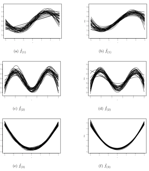
For illustration in Figure 5 the Mixed Model approach to smooth components (MM) is com-pared with BoostMixed for 30 datasets. It is seen that both methods detect the underlying smooth functions fairly well. However, it is seen that the mixed model approach has higher variability. For example for some datasets the componentf(1) has been strongly oversmoothed

yielding straight lines (rather than thesin function).

−3 −2 −1 0 1 2 3 −1.5 −1.0 −0.5 0.0 0.5 1.0 1.5 x Effect (a) ˆf₍₁₎ −3 −2 −1 0 1 2 3 −1.5 −1.0 −0.5 0.0 0.5 1.0 1.5 x Effect (b) ˆf₍₁₎ −2 0 2 4 6 8 −1.5 −1.0 −0.5 0.0 0.5 1.0 1.5 x Effect (c) ˆf₍₂₎ −2 0 2 4 6 8 −1.5 −1.0 −0.5 0.0 0.5 1.0 1.5 x Effect (d) ˆf₍₂₎ −3 −2 −1 0 1 2 3 −4 −2 0 2 4 6 x Effect (e) ˆf₍₃₎ −3 −2 −1 0 1 2 3 −4 −2 0 2 4 6 x Effect (f) ˆf₍₃₎

Figure 5: Thirty functions computed with mixed model methods(left panels) and boosting (right panels) (c= 1, p= 3)

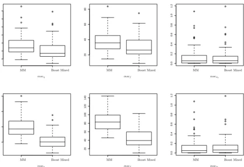
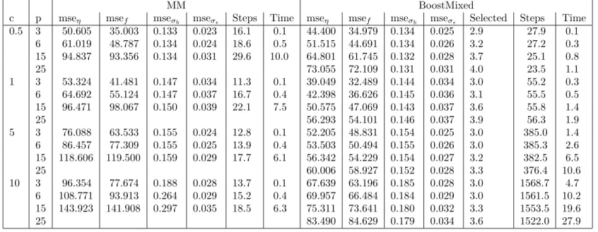
In Tables 1 and 2 the resulting mean squared errors are given for the low correlation case (ρ = 0.1) and the medium correlation case (ρ = 0.5). It is seen that for all components mean squared errors are smaller when BoostMixed is used. The difference is rather large for high dimensional predictors which include noisy covariates. BoostMixed then has the advantage that it automatically selects the right predictors. The number of selected predictors as given in Table 1 and 2 has mean values between three and four, thus showing that selection was successful.

20 40 60 80 100 120 140 50 100 150 200 20 40 60 80 20 40 60 80 100 120 140 0.0 0.2 0.4 0.6 0.8 1.0 1.2 0.0 0.2 0.4 0.6 0.8 1.0 1.2 MM MM MM MM MM MM Boost Mixed Boost Mixed Boost Mixed Boost Mixed Boost Mixed Boost Mixed mseη mseη msef msef mseσb mseσb

Figure 6: Boxplot for mseη, msef and mseσbadditive simulation study with c = 1 and p= 3

(top) andc= 1 and p= 15 (bottom)

50 100 150 l1 50 100 150 200 250 l1 20 40 60 80 100 120 140 l2 50 100 150 200 l2 0 4 l3 0 4 l3 MM MM MM MM MM MM Boost Mixed Boost Mixed Boost Mixed Boost Mixed Boost Mixed Boost Mixed mse η mse η mse f mse f mse σ b mse σ b

Figure 7: Boxplot formseη, msef andmseσb additive simulation study withc = 10 andp= 3

MM BoostMixed

c p mseη msef mseσb mseσǫ Steps Time mseη msef mseσb mseσǫ Selected Steps Time

0.5 3 48.919 37.610 0.119 0.028 14.7 0.14 44.178 38.435 0.114 0.026 2.9 21 0.13 6 59.117 48.360 0.119 0.029 17.9 0.52 51.380 47.964 0.112 0.028 3.2 21 0.27 15 92.049 85.762 0.127 0.031 26.2 9.01 60.406 58.639 0.111 0.028 3.6 20 0.72 25 70.528 70.860 0.108 0.030 3.8 19 0.93 1 3 54.240 37.535 0.124 0.024 11.0 0.10 41.470 30.457 0.119 0.026 3.0 61 0.35 6 63.671 48.900 0.118 0.024 15.4 0.45 45.094 34.757 0.119 0.027 3.2 61 0.64 15 97.211 85.477 0.120 0.028 21.4 7.36 53.980 45.249 0.121 0.030 3.7 62 1.62 25 62.094 55.092 0.118 0.032 4.0 81 2.59 5 3 74.485 60.585 0.186 0.032 12.9 0.12 51.907 46.045 0.181 0.030 3.0 456 1.66 6 85.335 72.724 0.185 0.031 14.3 0.42 52.756 47.277 0.181 0.031 3.0 457 3.25 15 119.919 114.034 0.188 0.036 20.2 6.97 57.385 53.415 0.177 0.035 3.2 464 8.94 25 61.299 58.286 0.176 0.038 3.4 464 13.43 10 3 91.144 71.836 0.264 0.026 13.8 0.13 62.942 60.312 0.140 0.029 3.0 1834 5.51 6 101.424 83.810 0.186 0.026 15.1 0.44 64.687 62.413 0.131 0.029 3.0 1833 12.38 15 135.990 126.305 0.197 0.034 19.5 6.76 70.245 69.627 0.137 0.034 3.3 1814 22.03 25 77.409 78.312 0.138 0.036 3.6 1812 32.19

Table 1: Comparison between additive mixed model fit and BoostMixed (ρ= 0.1).

MM BoostMixed

c p mseη msef mseσb mseσǫ Steps Time mseη msef mseσb mseσǫ Selected Steps Time

0.5 3 50.605 35.003 0.133 0.023 16.1 0.1 44.400 34.979 0.134 0.025 2.9 27.9 0.1 6 61.019 48.787 0.134 0.024 18.6 0.5 51.515 44.691 0.134 0.026 3.2 27.2 0.3 15 94.837 93.356 0.134 0.031 29.6 10.0 64.801 61.745 0.132 0.028 3.7 25.1 0.8 25 73.055 72.109 0.131 0.031 4.0 23.5 1.1 1 3 53.324 41.481 0.147 0.034 11.3 0.1 39.049 32.489 0.144 0.034 3.0 55.2 0.3 6 64.692 55.124 0.147 0.037 16.7 0.4 42.398 36.626 0.145 0.036 3.1 55.5 0.5 15 96.471 98.067 0.150 0.039 22.1 7.5 50.575 47.069 0.143 0.037 3.6 55.8 1.4 25 56.293 54.101 0.146 0.037 3.9 56.3 1.9 5 3 76.088 63.533 0.155 0.024 12.8 0.1 52.205 48.831 0.154 0.025 3.0 385.0 1.4 6 86.457 77.309 0.155 0.025 13.9 0.4 53.503 50.494 0.155 0.026 3.0 385.3 2.6 15 118.606 119.500 0.159 0.029 17.7 6.1 56.342 54.229 0.154 0.027 3.2 382.5 6.5 25 60.006 58.927 0.152 0.028 3.3 376.4 10.6 10 3 96.354 77.674 0.188 0.028 13.7 0.1 67.639 63.196 0.185 0.028 3.0 1568.7 4.7 6 108.771 93.913 0.264 0.029 15.2 0.4 69.957 66.484 0.184 0.029 3.0 1561.5 10.2 15 143.923 141.908 0.297 0.035 18.5 6.3 75.311 73.641 0.180 0.032 3.3 1553.5 19.6 25 83.490 84.629 0.179 0.034 3.6 1522.0 27.9

Table 2: Comparison between additive mixed model fit and BoostMixed (ρ= 0.5).

But it should be noted that also in the case where only the variables are included which carry information, the mean squared errors are still smaller when BoostMixed is used. For higher number of predictors (p>20) the Mixed Model fit did not work, therefore no values are shown in Table 1 and 2. The strongest reduction in terms of mean squared error is found for the estimation ofmseη the effect becomes stronger with increasing signalcand parametersp, see for example

mseη= 41.470 for BoostMixed andmseη = 54.240 for the additive model withc= 1, p= 3. In

Figure 6 and 7 the mean squared errors are given for the pure information case (p=3) and the case that includes several noise variables (p=15).

3.5

Application to CD4 data

For the AIDS Cohort Study MACS we considered the semi-parametric mixed model from Section 1

yit=µparit +µaddit +bit+ǫit,

whereyitdenotes the square root CD4 number of cells for subjection measurementt(taken at

irregular time intervals). The parametric and nonparametric term are given by µpar_i = β0+drugsiβD+partnersiβP,

µadd

it = αT(time) +αA(agei) +αC(cesd).

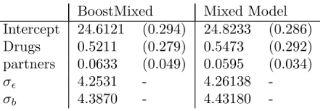
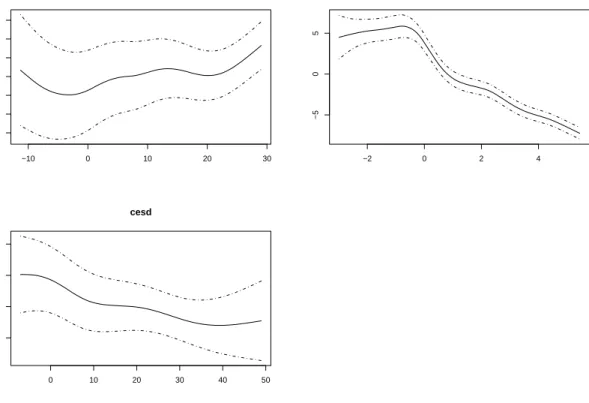
where cesd is a mental illness score. The square root transformation has been used since the original CD4 cell number varies over a wide range. This is a kind of stabilization transformation for variances. The estimated effect of time was modelled smoothly with the resulting curve given in Figure 1. This smooth curve can be compared to the results of Zeger & Diggle (1994) who applied generalized estimation equations. In Figure 8 the smooth effects of age, the mental illness score and time are given. It is seen that there is a slight increase in CD4 cells for increasing age and a decease with higher values of the mental illness score. Table 3 shows the estimates for the parameters. Comparison between BoostMixed and the mixed model approach shows that the estimates are well comparable.

BoostMixed Mixed Model Intercept 24.6121 (0.294) 24.8233 (0.286) Drugs 0.5211 (0.279) 0.5473 (0.292) partners 0.0633 (0.049) 0.0595 (0.034) σǫ 4.2531 - 4.26138

-σb 4.3870 - 4.43180

-Table 3: Estimates for the AIDS Cohort Study MACS with BoostMixed and mixed model approach (standard deviations given in brackets)

4

Random slopes on smooth effects

4.1

Estimation by boosting techniques

The semiparametric additive model (3) allows for additive effects of covariates, including multi-variate random effects. For example random slopes for linear terms are already included. With wit=xit model (3) becomes yit= m X j=1 α(j)(uitj) +xTitβ+xTitbi+εit

−10 0 10 20 30 −1.5 −0.5 0.5 1.0 1.5 age 0 10 20 30 40 50 −1 0 1 2 cesd −2 0 2 4 −5 0 5 time

Figure 8: Estimated effect of age, the illness score cesd and time based on BoostMixed andbirepresents random slopes on the variablesxit. Quite a different challenge is the

incorpora-tion of random effects in additive terms. For simplicity of presentaincorpora-tion we restrict consideraincorpora-tion to one smooth effect. Let the smooth random intercept model

yit=β0+α(ui) +bi0+εit, bi0∼N(0, σ2),

be extended to

yit=β0+α(ui) +α(ui)bi1+bi0+εit, (11)

with bi0, bi1∼N(0, Q(ρ)).

As usual the smooth component has to be centered for reasons of identifiability of effects, in our applicationsP

iα(ui) = 0 has been used. That means the ”random slope”bi1in model (11) is a

parameter that, quite similar to random slopes in linear mixed models, lets the strength of the variable vary across subjects. The dependence on variableui becomes

α(ui) +α(ui)bi1=α(ui)(1 +bi1)

showing thatα(ui) represents the basic effect of variable ui but this effect can be stronger for

individuals ifbi1>0 and weaker if bi1 <0. Thusbi1 strengthens or attenuates the effect of the

variableui. If the variance of bi1 is very large it may even occur thatbi1 <1 meaning that the

effect ofui is ”inverted” for some individuals. Ifα(ui) is linear with α(ui) =βui, the influence

term is given byα(ui)(1 +bi1) =ui(β+ ˜bi1) where ˜bi1=βbi1represents the usual term in linear

mixed models with random slopes. Thus comparison with the linear mixed model should be based on the rescaled random effect ˜βi1 withE( ˜βi1) = 0,Var( ˜βi1) =β2Var(βi1).

The main problem in model (11) is the estimation of the random effect. Ifα(u) is expanded in basis functions byα(u) =P

sαsΦs(u) one obtains

α(ui)bi= X

s

which is a multiplicative model sinceαsand bi are unknown and cannot be observed. However,

boosting methodology may be used to obtain estimates for the model. The basic concept in boosting is that in one step the refitting ofα(ui) is done by using a weak learner which in our

case corresponds to largeλin the penalization term.

Thus in one step the change from iteration α(l)_{to α}(l+1) _{is small. Consider model in vector}

form with predictor

ηi=1β0+ Φiα+ (1Φiα) bi bi1 where 1T _{= (1, . . . ,1) is a vector of 1s, Φ}

i is the corresponding matrix containing evaluations of

basis functions and αT _{= (α}

1, . . . αn) denotes the corresponding weights. Then the refitting of

residuals in the iteration step is modified in the following way. Letη(l−1)

i denote the estimate from the previous step. Then the refitting of residuals (without

selection) is done by fitting the model yi−η(l −1) i ∼N(ηi, Vi(θ)) with ηi=1β0+ Φiα+ (1,Φiαˆ(l−1)) bi0 bi1 (12) whereβ0, αare the parameters to be estimated and the estimate from the previous step ˆα(l−1)is

considered as known parameter. With resulting estimates ˆβ0,αˆ the corresponding update step

takes the form

ˆ

α(l)= ˆα(l−1)

+ ˆα , βˆ₀(l)= ˆβ(l−1)

0 + ˆβ0.

The basic idea behind the refitting is that forward iterative fitting procedures like boosting are weak learners. Thus the previous estimate is considered as known in the last term of (12). Only the additive term Φiαis refitted within one iteration step. Of course after the refit the variance

components corresponding to (bi0, bi1) have to be estimated.

4.2

Application to Jimma Study

For the Jimma data from Section 1 we focus on the effect of age (in days) on the weight of children. Since growth measurements usually do not evolve linearly in time the use of a linear mixed model involves to find an appropriate scale of age. Lesaffre, Asefa & Verbeke (1999) found that weight is approximately linearly related with the square root of age. An even better approximation, they actually used in their analysis is the transformation (age−log(age+ 1)−0.02×age)1/2_.

Since in growth curve analysis random slopes are needed , they had to find the scale before using mixed model methodology. The big advantage of the approach proposed here is that the scale of age has not to be found separately but is determined by the (flexible) mixed model itself. The model we consider includes random slopes on the age effects, smooth effect of age of mother and several parametric terms for the categorical variables. It has predictor

ηit=β0+αA(Agei) +bi0+bi1αA(Agei) +αAM(Age of M otheri) + parametric term.

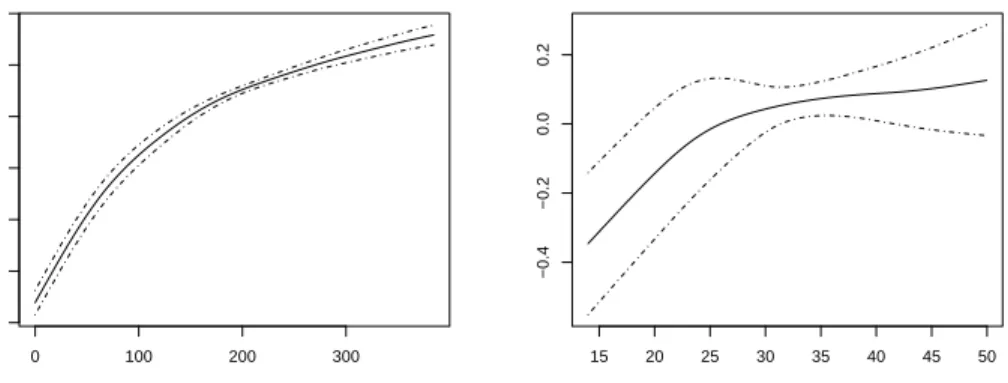
Figure 3 shows the overall dependence (of children). Figure 9 shows the (centered) dependence on age and age of mother. It is seen that the effect of age of mothers is hardly linear (as assumed in the linear mixed models). Body weight of children seems to increase with age of mother up to about 30 years, then the effect remains rather stable. Table 4 gives the estimates of the parametric terms. For comparison the estimates for the linear mixed model with random slopes on the transformed age and linear effect of age of mother are given in Table 4 . As transformed age we use (age−log(age+ 1)−0.02×age)1/2_{as suggested by Lesaffre, Asefa & Verbeke (1999).}

0 100 200 300 −4 −3 −2 −1 0 1 2 Age of children 15 20 25 30 35 40 45 50 −0.4 −0.2 0.0 0.2 Age of Mother

Figure 9: Effects of age of children (in days) and age of the mother (in years) in the Jimma study intercepts are due to centering of variables. For age of mother the linear model shows a distinct increase ( 0.014 with standard deviation 0.004 ).

Table 5 shows the estimated variance of (bi0, bi1) for the flexible model and the linear mixed

model with transformed age.

BoostMixed Mixed Model INTER 6.819 0.174 2.664 0.176 SEX 0.304 0.049 0.296 0.081 EDUC0 -0.051 0.066 -0.085 0.118 EDUC1 -0.021 0.151 -0.044 0.236 EDUC2 0.041 0.051 0.009 0.093 EDUC3 0.036 0.029 -0.005 0.060 EDUC4 -0.005 0.019 -0.042 0.042 VISIT -0.078 0.072 -0.078 0.117 TIME -0.177 0.065 -0.169 0.107 DELIV1 -0.027 0.007 -0.019 0.010 DELIV2 -0.148 0.031 -0.141 0.052 AGE 0.886 0.004 AGEM 0.014 0.004

Table 4: Effects of categorical covariates in Jimma study

BoostMixed Mixed Model 0.825962 0.196618 0.171369 -0.017506 0.196618 0.057253 -0.017506 0.045134

Table 5: Covariance matrix for random intercept and slope for Jimma data

5

Some Extensions

By allowing the variables u1, . . . , um to have additive form model (3) represents a partially

additive mixed model. More flexible predictors have been proposed in regression models, in particular varying coefficients models (Hastie & Tibshirani (1993)) and interactions between covariates. In the following the extension to more flexible forms of predictors in mixed models is considered briefly. For simplicity we consider only one additional term and variables that do not

vary across replications. The effect of variablezi varies with variableui within a mixed model

framework if the (additional) nonparametric term is given by µnonp.it =α(ui) +ziγ(ui),

whereα(ui) andγ(ui) are unspecified functions of the continuous variableuiHastie & Tibshirani

(1993) call ui an effect modifier since the effect ofzi depends on the value of ui. Often zi is a

factor represented by a 0-1 dummy variable. The (simplified) model has the form yit = µnonp.it +µrandit +εit

= α(ui) +ziγ(ui) +witTbi+εit

which in general is enlarged by further linear and additive terms. For the vector representation one obtains

yi= Φiα+ Φi(zi)γ+Wibi+εi

where Φi represents the basis function for the additive termα(ui) (see Section 2.1) and Φi(z) is

a matrix composed from observationsz and basis functions forγ(ui). Let γ(u) be represented

by γ(u) = n X s=1 γsΦ(sz)(u),

then one obtains

ziγ(ui) = n X s=1

γsziΦ(sz)(ui)

and the matrix Φi(z) = (Φrs) has elements Φrs = zrΦ(5z)(ur). The corresponding vector γ is

given byγT _{= (γ}

1, . . . γM). Thus the model has the form (4) and may be estimated by boosting.

After the additive terms have been fitted, the varying coefficients term Φi(zi)γ is included by

fitting in Step 2 of the algorithm the model for residuals yi−η(l

−1)

i ∼N(Φi(zi)γ, Vi(θ))

yielding an estimate for γ. If one wants to consider more candidates for varying coefficients a selection step should be included.

6

Concluding Remarks

Alternative estimates have been proposed that yield stable estimates of additive mixed models also in the high dimensional case. If additive structures with a random intercept are not sufficient to capture the variation across subjects it is recommended to include an additional random slope which strengthens or attenuates the effect of a covariate. The model with random slopes is simply structured and adds only two additional parameters, the variance of the slope and the covariance between slope and intercept. It is therefore very parsimonious and allows simple interpretation. By using few additional parameters it has a distinct advantage over methods that allows subjects to have their own function, yielding as many functions as subjects (see Verbyla, Cullis, Kenward & Welham (1999)).

Acknowledgement

We gratefully acknowledge support from Deutsche Forschungsgemeinschaft ( Sonderforschungs-bereich 386: Diskrete Strukturen ). We thank Emannuel Lesaffre for letting us use the Jimma data.

A

Appendix

A.1

ML for Variance Components

The estimation of the variance components is based on the profile log-likelihood that is obtained by plugging in the estimates ˆδfrom a fixed boosting step in the penalized log-likelihood.

l(ˆδ;θ) =−1 2 Pn i=1log(|Vi(θ)|) +Pni=1(yi−ηˆTVi(θ)−1(yi−η)ˆ −1 2δ T_Kδ.

Differentiation with respect toθT _{= (σ}

ε, ̺T) = (θ1, . . . , θd) yields s(ˆδ, θ) = ∂l(ˆ_θδ,θ) = (s(ˆδ, θ)i)i=1,...,d and F(ˆδ, θ) =−E(∂_∂θ∂θ2l(ˆδ,θT)) = (F(ˆδ, θ)i,j)i,j=1,...,d with s(ˆδ, θ)i=∂l(ˆ_θiδ,θ) = −1₂Pnk=1trace (Vk(θ)) −1∂Vk(θ) θi +1₂Pn k=1(yk−η(l))TVk(θ)−1∂Vk_θi(θ)Vk(θ)−1(yk−η(l)) and F(ˆδ, θ)i,j= 1 2 n X k=1 trace (Vk(θ)) −1∂Vk(θ) ∂θi (Vk(θ)) −1∂Vk(θ) ∂θj where ∂Vk(θ) ∂θi = ( 2σITk ifi= 1 Wk∂Q_∂θj(̺)WkT ifj =i, i6= 1.

It should be noted that maximization ofl(ˆδ, θ) ignores the penalty term forδ. For example, in the case of independence

Q(̺) =̺2∗I the elementwise derivative is

∂Q(̺)

∂̺ = 2̺∗I.

The estimator ˆθcan now be obtained by running a common Fisher scoring algorithm with ˆ

θ(s+1)_{= ˆθ}(s)_{+F(ˆδ, θ}(s)_,)−1_s(ˆδ,θˆ(s)₎

wheres denotes the iteration index of the Fisher scoring algorithm. If Fisher scoring has con-verged the resulting ˆθ represents the estimates of variances for the considered boosting step.

A.2

Replacing the Truncated Power Series by B-Splines

In the following the use of B-Splines is sketched. For simplicity only one smooth component is considered with Φ1(u), . . . ,ΦM(u) denoting the B-Splines for equidistant knots k1, . . . , kM and

ηi=Ziβ+ Φiαdenoting the predictor.

Let us first consider the difference matrix Dd _{corresponding to B-Spline penalization (see}

Eilers & Marx (1996)). WithDbeing the (M −1)×M contrast matrix

D=      −1 1 −1 1 . .. ... −1 1     

one obtains higher order differences by the recursion Dd _{= DD}d−1 _{which is a (M −d)×M}

matrix. The penalty term is based on ˜K = (Dd₎T_Dd_{. New matrices ˜X}

(d), depending on the

order of the penalized differences are defined by

˜ X(1)=    1 .. . 1   , ˜ X(2)=    1 k1 .. . ... 1 kM   , ˜ X(3) =    1 k1 k21 .. . ... ... 1 kM k2M   .

For differences of order d one consider the (M−d)×M matrix ˜WT

(d)= (Dd(Dd)T)

−1_Dd_{.In the}

following we drop the notation of d and setD:=Dd_{, ˜W := ˜W}

(d)and ˜X:= ˜X(d). So ˜W and ˜Xhave

the propertiesDX˜ = 0, ˜WT_{X˜ = (DD}T₎−1_{DX˜ = 0, ˜X}T_{KX˜ = 0 = ˜X}T_DT_{DX˜ = (DX)˜} T_(DX˜).

Most important is the equation ˜

WTKW˜ = (DDT)−1

DDTDDT(DDT)−1

=I(M−d).

Since ˜WT_{X˜ = 0,αcan be decomposed intoα= ˜Xϕ+ ˜Wα.˜}

The predictor can now be rewritten in the form ηi =Zi,Φi β α +Wibi=Zi,Φi β ˜ Xϕ+ ˜Wα˜ +Wibi = Zi,ΦiX,˜ ΦiW˜   β ϕ ˜ α  +Wibi = Zi,ΦiX˜ β ϕ + ΦiW , W˜ i ˜ α bi .

The penalized log-likelihood of the linear mixed model simplifies to lp(δ) =Pni=1log(f(yi|δ;bi)p(bi))−λδTDiag(0(p×p), λK)δ

=Pn

i=1log(f(yi|δ;bi)p(bi))−λ(( ˜Xϕ+ ˜Wα)˜ TK( ˜Xϕ+ ˜Wα)˜

=Pn

i=1log(f(yi|δ;bi)p(bi))−₂1α˜T2∗λI(M−d)α.˜

This corresponds to the BLUP criterion of the mixed model yi= ˜Ziβ˜+ΦiW˜ W ˜ α bi +ǫi with   ˜ α bi ǫ  ∼N     0 0 0  ,   1 2λI 0 0 0 Q(ρ) 0 0 0 σ2 ǫI     and ˜βT _{= (β}T_{, ϕ}T_{), ˜Z}

i = [Zi,ΦiX]. Thus, from decomposition˜ α= ˜Xϕ+ ˜Wα˜ one obtains a

mixed model with uncorrelated parameters ˜α.

References

Breiman, L. (1999). Prediction games and arcing algorithms. Neural Computation 11, 1493– 1517.

Brumback, B. A. and Rice, J. A. (1998). Smoothing spline models for the analysis of nested and crossed samples of curves.Journal of the American Statistical Association93, 961–976. B¨uhlmann, P. and Yu, B. (2003). Boosting with l2 loss: Regression and classification.Journal

Dettling, M. and B¨uhlmann, P. (2003). Boosting for tumor classification with gene expression data.Bioinformatics 19, 1061–1069.

Eilers, P. H. C. and Marx, B. D. (1996). Flexible smoothing with B-splines and penalties. Statistical Science 11, 89–121.

Fahrmeir, L. and Lang, S. (2001). Bayesian inference for generalized additive mixed models based on Markov random field priors.Applied Statistics (to appear).

Friedman, J. (2001). Greedy function approximation: a gradient boosting machine.Annals of Statistics 29, 337–407.

Green, D. J. and Silverman, B. W. (1994). Nonparametric Regression and Generalized Linear Models: A Roughness Penalty Approach. London: Chapman & Hall.

Harville, D. A. (1974). Bayesian inference for variance components using only error contrasts. Biometrika 61, 383–385.

Harville, D. A. (1977). Maximum likelihood approaches to variance component estimation and to related problems.Journal of the American Statistical Association 72, 320–338.

Hastie, T. and Tibshirani, R. (1990).Generalized Additive Models. London: Chapman & Hall. Hastie, T. and Tibshirani, R. (1993). Varying-coefficient models.Journal of the Royal

Statis-tical Society B 55, 757–796.

Henderson, C. R. (1953). Estimation of variance and covariance components. Biometrics 9, 226–252.

Kaslow, R. A., Ostrow, D. G., Detels, R., Phair, J. P., Polk, B. F., and Rinaldo, C. R. (1987). The multicenter aids cohort study: Rationale, organization and selected characteristic of the participiants.American Journal of Epidemiology 126, 310–318.

Laird, N. M. and Ware, J. H. (1982). Random effects models for longitudinal data. Biomet-rics 38, 963–974.

Lesaffre, E., Asefa, M., and Verbeke, G. (1999). Assessing the goodness-of-fit of the laird and ware model - an example: The jimma infant survival differential longitudinal study. Statistics in Medicine 18, 835–854.

Lin, X. and Zhang, D. (1999). Inference in generalized additive mixed models by using smooth-ing splines.Journal of the Royal Statistical Society B61, 381–400.

Marx, D. B. and Eilers, P. (1998). Direct generalized additive modelling with penalized likeli-hood.Comp. Stat. & Data Analysis 28, 193–209.

McCulloch, C. E. and Searle, S. R. (2001). Generalized, linear and mixed models. New York: Wiley.

Parise, H., Wand, M. P., Ruppert, D., and Ryan, L. (2001). Incorporation of historical controls using semiparametric mixed models.Applied Statistics 50, 31–42.

Patterson, H. and Thompson, R. (1974). Maximum Likelihood Estimation of Components of Variance. Proceedings of the 8th International Biometric Conference.

Robinson, G. K. (1991). That BLUP is a good thing: The estimation of random effects (with discussion).Statistical Science 6, 15–51.

Ruppert, D. and Carroll, R. J. (1999). Spatially-adaptive penalties for spline fitting.Australian Journal of Statistics 42, 205–223.

Schimek, M. (2000). Smoothing and Regression. Approaches, Computation and Application. New York: Wiley.

Speed, T. (1991). That BLUP is a good thing: The estimation of random effects: Comment. Statistical Science 6, 42–44.

Verbeke, G. and Molenberghs, G. (2001). Linear Mixed Models for Longitudinal Data. New York: Springer.

Verbyla, A. P., Cullis, B. R., Kenward, M. G., and Welham, S. J. (1999). The anlysis of de-signed experiments and longitudinal data by using smoothing splines.Applied Statistics48, 269–311.

Wand, M. P. (2000). A comparison of regression spline smoothing procedures.Computational Statistics 15, 443–462.

Wand, M. P. (2003). Smoothing and mixed models.Computational Statistics 18, 223–249. Wood, S. N. (2004). Stable and efficient multiple smoothing parameter estimation for

gener-alized additve models.Journal of American Statistical Association 99, 673–686.

Zeger, S. L. and Diggle, P. J. (1994). Semiparametric models for longitudinal data with appli-cation to cd4 cell numbers in hiv seroconverters.Biometrics50, 689–699.

Zhang, D., Lin, X., Raz, J., and Sowers, M. (1998). Semi-parametric stochastic mixed models for longitudinal data.Journal of the American Statistical Association 93, 710–719.