System GMM Estimation With A Small Sample

(1)

SYSTEM GMM ESTIMATION WITH A SMALL SAMPLE

Marcelo Soto July 2009

Properties of GMM estimators for panel data, which have become very popular in the empirical economic growth literature, are not well known when the number of individuals is small. This paper analyses through Monte Carlo simulations the properties of various GMM and other estimators when the number of individuals is the one typically available in country growth studies. It is found that, provided that some persistency is present in the series, the system GMM estimator has a lower bias and higher efficiency than all the other estimators analysed, including the standard first-differences GMM estimator.

Keywords: Economic Growth, System GMM estimation, Monte Carlo Simulations JEL classification: C15, C33, O11

_{Institut d'Anàlisi Econòmica, Barcelona. Email: [email protected]. I am grateful to Richard}

Blundell, Frank Windmeijer and participants in the Econometric Society meetings in Mexico DF and Wellingtron for comments and helpful suggestions. The support from the Spanish Ministry of Science and Innovation under project ECO2008-04837/ECON is gratefully acknowledged. The author acknowledges the support of the Barcelona GSE Research Network and of the Government of Catalonia.

(2)

1. Introduction

The development and application of Generalised Methods of Moments (GMM) estimation for panel data has been extremely fruitful in the last decade. For instance, Arellano and Bond (1991), who pioneered the applied GMM estimation for panel data, have more than 1,200 citations according to ISI Web of Knowledge as of July 2009.

In the empirical growth literature, GMM estimation has become particularly popular. The Arellano and Bond (1991) estimator in particular initially benefited from widespread use in different topics related to growth1_{. Subsequently the related Blundell and Bond (1998)}

estimator has gained an even grater attention in the empirical growth literature2_.

However, these GMM estimators were designed in the context of labour and industrial studies. In such studies the number of individuals N is large, whereas the typical number of cross-units in economic growth samples is much smaller. Indeed, availability of country data limits N to at most 100 and often to less than half that value.

The lack of knowledge about the properties of GMM estimators when N is small renders them a sort of a black box. Moreover, a practical problem not addressed in the earlier literature refers to fact that the low number of cross-units may prevent the use of the full set of instruments available. This implies that, in order to make estimation possible, the number of instruments must be reduced. The performance of the various GMM estimators in panel data is not well known when only a partial set of instruments is used for estimation.

This paper analyses through Monte Carlo simulations the performance of the system GMM and other standard estimators when the number of individuals is small. The simulations follow closely those made by Blundell et al (2000) in the sense that the structure of the model simulated is exactly the same as theirs. The only difference is that Blundell et al. chose N=500, while this paper reports results for N more adapted to the actual sample size of growth regressions in a panel of countries (N=100, 50, 35). A small N constrains the researcher to limit the number of instruments used for estimation, which may also have a consequence on the properties of the estimators. The paper studies the behaviour of the estimators for different choices on the instruments.

1_{For instance Caselli et al (1996) use it to test the Solow model; Greeanway et al (2002) for} analysing the impact of trade liberalisation in developing countries; and Banerjee and Duflo (2003) to investigate the effect of income inequality on growth.

2_{Some examples are studies on aid and growth (Dalgaard et al, 2004); education and growth} (Cohen and Soto, 2007); and exchange rate volatility and growth (Aghion et al, 2009).

(3)

The next section depicts the econometric model under consideration. Section 3 presents the estimation results obtained by Monte Carlo simulations. Section 4 concludes.

2. The econometric model

We will consider an autoregressive model with one additional regressor:

it i it 1 it it

α

y

β

x

η

u

y







(1)

for i = 1,…, N and t = 2,…, T, with

α



1

.The disturbances

η

_i and u_it have the standard properties. That is,

 

η

_i



0 ,

E

 

u

_it



0 ,

E



η

_i

u

_it





0 E

for i = 1,…, N and t = 2,…, T. (2)

Additionally, the time-varying errors are assumed uncorrelated:



u

_is

u

_it





0 E

for i = 1,…, N and  t  s. (3)

Note that no condition is imposed on the variance of uit, hence the moment conditions

used below do not require homoskedasticity.

The variable xit is also assumed to follow an autoregressive process:

it it i 1 it it

x

τη

θ

u

e

x









(4)

for i = 1,…, N and t = 2,…, T, with





1

. The properties of the disturbance eit are

analogous to those of uit. More precisely,

 

e

_it



0 ,

E



η

_i

e

_it





0 E

for i = 1,…, N and t = 2,…, T. (5)

Two sources of endogeneity are present in the xit process. First, the fixed-effect component

_i has an effect on xit through a parameter  implying that yit and xit have both a steady

state determined only by i. And second, the time-varying disturbance uit impacts xit with a

parameter . A situation in which the attenuation bias due to measurement error predominates over the upward bias due to simultaneity determination may be simulated with < 0.

For simplicity, it is useful to express xit and yit as deviations from their steady state values.

(4)

may be written as a deviation from its steady state: it i it

₁

ξ

τη

x









(6)

where the deviation from steady state

ξ

_it is equal to



 

1 _it _it



it

1 L

θ

u

e

ξ











.

In this last expression L is the lag operator and so, for any variable wit and parameter , (1

L)1_w it is defined as

...

2 -it 2 1 -it it it 1

_w

_λ

_w

_λ

_w

λ

L)

(1







Similarly, assuming that (1) is a valid representation of yit for t = 1,…, 



, we have,

it 1 it 1 i it

₁

η

_α

β(1

αL)

x

(1

αL)

u

y











After substituting in this last expression x_it by (6), y_it may be written as











i it it

η

ζ

1 α

1 βτ

1 y















(7)

with its deviation from steady state given by,





1 _it it it 1 1 it

β

(1

α

L)

(1

L)

θ

u

e

(1

α

L)

u

ζ













 .

Hence, the deviation it from the steady state is the sum of two independent AR(2)

processes and one AR(1) process.

3. Monte Carlo simulations

This section reports Monte Carlo simulations for the model described in (1) to (5) and analyses the performance of different estimators. To summarise, the model specification is:

it i it 1 it it

α

y

β

x

η

u

y



_



(8)

(5)

it it i 1 it it

x

τη

θ

u

e

x





_



(9) with

)

;

0 (

~

);

;

0 (

~

);

;

0 (

~

2_η _it 2_u _it _e2 i

σ

u

σ

e

σ

η

N

.

We will consider three different cases for the autoregressive processes: no persistency (=

 = 0), moderate persistency (=  = 0.5) and high persistency (=  = 0.95). The other parameters are kept fixed in each simulation as follows3_:

 = 1;  = 0.25;  = 0.1;

σ

_η2



1;

σ

2_u



1;

σ

2_e



0.16

.

The parameter  is negative in order to emulate the effects of measurement error in xit4.

The hypothesis of homoskedasticity is dropped in subsequent simulations. Initially, the sample size considered is N = 100 and T = 5. In later simulations N is set at 50 and 35 with T=12, in order to illustrate the effects of a low number of individuals (relative to T). Each result presented below is based on a different set of 1000 replications, with new initial observations generated for each replication. The appendix A explains with more details the generation of initial observations.

The estimators analysed are OLS, fixed-effects, difference GMM, level GMM and system GMM. One and two-step results are reported for each GMM estimation. All the estimations are performed with the program DPD for Gauss (Arellano and Bond, 1998).

3.1 Accuracy and efficiency results

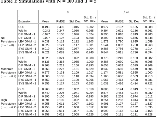
The main finding is that, provided that some persistency is present in the series, the system GMM estimator yields the results with the lowest bias. Consider Table 1, which presents results for N=100 and T=5. The performance of each estimator varies according to the degree of persistency in the series. For instance, when  and  are both equal to zero, OLS estimates wrongly assign a highly significant coefficient to the lagged dependent variable, whereas the Within estimator provides a negative and significant coefficient5_{. However,}

3_{These values are the same as those selected by Blundell et al (2000)}

4_{Hauk and Wacziarg (2009) carry out Monte Carlo simulations for the convergence equation} derived from the Solow model by directly introducing noise in the variables.

5_{Recall that the OLS coefficient on y}_it_₁_{is biased towards 1 and the Within groups coefficient is} biased downwards (with a bias decreasing with T).

(6)

OLS provides estimates for  with the lowest root mean square error (RMSE) in the no-persistency case6_{. The high RMSE on}__{displayed by all GMM estimates is a consequence}

of the weakness of the instruments for xit discussed in appendix B when  = 0.

In the moderate persistency case ( and  equal to 0.5), the OLS estimator has again a strong upwards bias for  and a downwards bias for . The Within estimator is strongly biased downwards in both cases. The difference GMM estimator results in coefficients between 60% and 70% the real parameter values and presents the highest RMSE for . This shows that lagged levels are weak instruments for variables in differences even in a moderate-persistency environment. As to the level and system GMM estimates, they display systematically the lowest bias for both  and . In addition, these estimators result in the lowest RMSE for .

In the high persistency case ( and  equal to 0.95), the system GMM estimator outperform all the other estimators in terms of bias and efficiency. Note however that the bias in the lagged dependent variable of the OLS estimator is considerably reduced. This is due to the fact that this coefficient is biased towards 1.

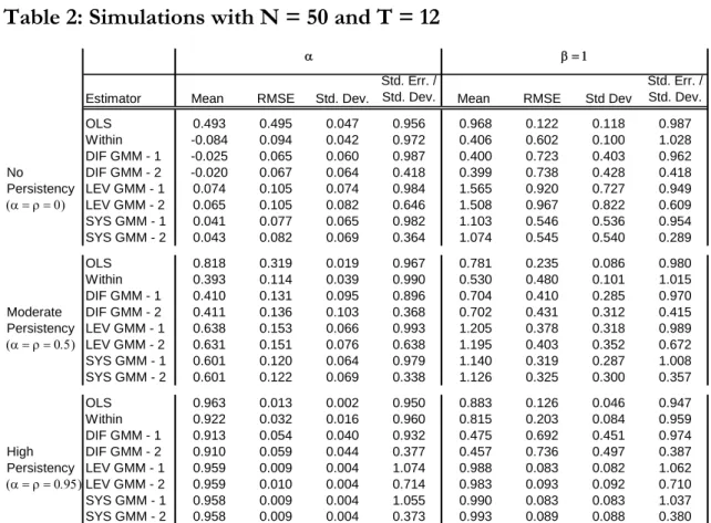
One well known caveat of GMM estimators refers to their reported two-step standard errors, which systematically underestimate the real standard deviation of the estimates (Blundell et al, 2000). For instance, standard errors of system GMM are 62% to 74% lower than the standard deviation of the estimates of  and 70% to 83% lower in the case of . This result suggests taking the one-step estimates for inference purposes, since accuracy and efficiency (measured by the RMSE) are similar to those of the two-steps. The variance correction suggested by Windmeijer (2005) is implemented in the current simulations. The next step is to replicate the Monte Carlo experiments by changing the sample sizes. Results are now obtained by setting N = 50 and T = 12. The reduction of N relative to T precludes the use of the full set of instruments derived from conditions (10) and (10). Indeed, if all those moment conditions were exploited the number of instruments would be (T2)(T+1), which exceeds N. On the other hand, the optimal weighting matrix W_S defined in (10) has a rank of N at most. Therefore, if the number of instruments exceeds N, WS is singular and the two-step estimator cannot be computed. In order to make

estimation possible only the most relevant (i.e. the most recent) instruments are used in

6_{The RMSE on}_{is defined as}











R 1 j j

β

R

1

2

(7)

each period. That means that only levels lagged two periods are used for the equation in differences and, as before, differences lagged one period are used for the equation in levels. This procedure results in 4(T2) instruments. The results are presented in Table 2.

The main conclusions are the same as those obtained from Table 1. That is, in the simulations without persistency, all the estimators perform badly. The OLS and fixed-effect estimators present considerable biases and, although the system GMM estimator displays a relatively low bias, it has a high RMSE for . As to the moderate and high-persistency cases, the system GMM does better than any other estimator overall. Still, the moderate-persistency estimation suffers from a small sample upwards bias of 20% for  and of 14% for .

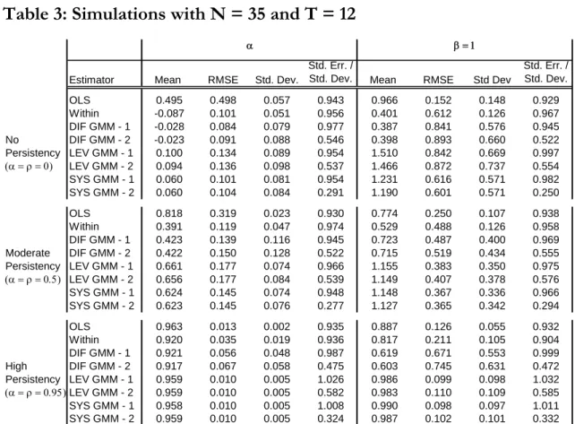
The next set of results is obtained by straining even more the sample size, with N = 35 and T = 12. From the previous discussion it becomes apparent that the system GMM estimation with the set of instruments used in the previous simulations is not feasible since the number of instruments 4×(122)=40 exceeds the number of individuals. Several alternatives were considered for reducing the number of instruments. First, lagged levels of x_it were omitted from the instrument set for the equation in differences and Z_l was kept as before. Second, lagged differences of xit were omitted from the instrument set for the

equation in levels and Zd was kept as before. And third, Zl was kept as before and Zd was

modified as follows,















  iT 2 i2 i1 2 iT i2 i1 di

x

y

0

0 



Z

(10)

Under this last alternative the total number of instruments is 3×(T2)+1=31. Although all three alternatives provided similar results in terms of bias, the third alternative resulted in the lowest RMSE error in the high-persistency case. Table 3 compares the different estimators, with the instruments for the system GMM estimator defined in (10) for the equation in differences and in (10) for the equation in levels. In general the RMSE are higher than in the previous simulations due to the smaller sample size. In addition, the upward bias for  obtained by system GMM is higher than before. But overall, this estimator outperforms in terms of accuracy and efficiency once again.

(8)

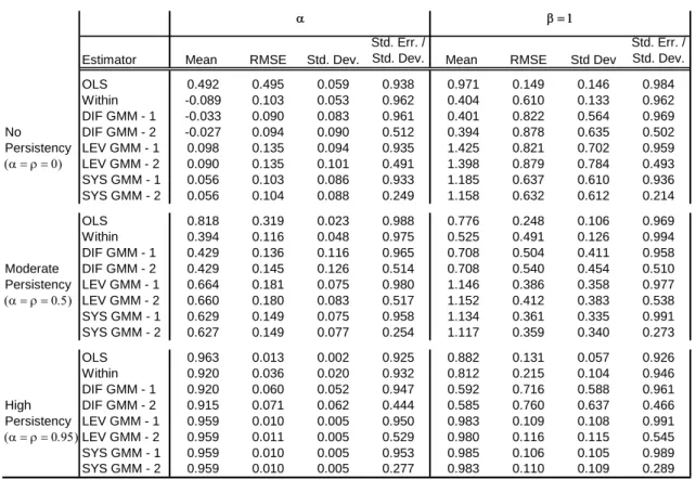
results presented in tables 1 to 3 are based on residuals with variances and . Now heteroskedasticity is introduced by generating residuals uit and eit such

that and . This particular structure implies that the

expected variances of uit and eit are the same as in the previous simulations and that the

ratio is constant, thus making easier the comparison with the results previously shown. Table 4 reports the simulation results with N = 35 and T =12. The instruments used correspond to those of Table 3. The main effect of heteroskedasticity is to slightly increase the RMSE of  in the high-persistency case. Still, the level and system GMM estimators display both the lowest finite-sample bias and the lowest RMSE.

1 σ

2_u



0.16 σ

2_e



σ

2_u i

~

U

2 ui

σ

/

1.5)

;

(0.5

2 ei 2 u 2 ei

0.16 σ

i

σ



Figure 1 presents the distribution of the estimates obtained with OLS, and one and two-step system GMM. The distributions correspond to the sample with N = 35, T = 12 and with heteroskedastic residuals across individuals. The vertical line corresponds to the parameter values. The figure shows that the distributions of the one and two-step system GMM are more concentrated around parameter than the distribution obtained from OLS. However, the GMM estimators are systematically biased upwards, though the bias is considerably lower than the one present in OLS. Regarding , the distributions of GMM estimates in the no-persistency case though centred on the right value have very fat queues. The OLS estimator performs better in this particular case. In the cases with moderate and high persistency the dispersion of GMM distribution is considerably reduced and its bias is systematically lower than OLS's.

One striking feature of GMM estimators is that the gain in efficiency from the two-step estimator is almost inexistent: the one and two step distributions are virtually the same. More work should be done in order find out the cases in which the two-step estimator does better than the one-step estimator.

3.2 Type-I error and power of significance tests.

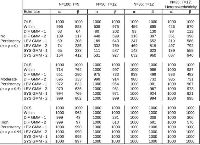
Another aspect in which the various estimators can be evaluated is the frequency of wrong rejections of the hypothesis that is not significant when it is in fact equal to zero (i.e. type-I error) and the power to properly reject lack of significance when coefficients are different from zero. Table 5 reports the frequency rejections at a 5% level of the hypothesis that  = 0 and  = 0 for the different simulations described above.

(9)

always rejects lack of significance, even in the case when  = 0 (see the no-persistency case). This is an additional flagrant implication of the upward bias of OLS estimates. A similar phenomenon occurs with the Within estimator, which fails to discard significance of  in 43% to 99.5% of the simulations with  = 0. As mentioned before, the standard error of two-step GMM estimators underestimate the real variability of the coefficients. A consequence of this is the relatively high number of wrong rejections of non-significance of  in the simulations with  = 0 in two-step GMM estimates (up to 69% in the system GMM estimator in the simulation with heteroskedasticity). The lowest type-I errors correspond to one-step GMM estimators, although they also tend to over-reject as N becomes smaller.

The weakness of the difference GMM estimator is reflected in its low power to reject non-significance when parameters are in fact different from zero. For instance, in the high-persistency case the one-step difference GMM estimator rejects non-significance of  in only 4% to 30% of the simulations that is, it wrongly dismisses the significance of  in 70% to 96% of the simulations. The system estimator is the most powerful among GMM estimators, with its power increasing as series become more persistent. For instance, according to one-step estimates in the heteroskedastic case, the non-significance of  was rejected in 56% of the simulations without persistency, 92% of simulations with moderate persistency, and 100% of simulations with high persistency.

Overall, the one-step system GMM is the more reliable estimator in terms of power and error type-I. Among all the estimators presented in the table, the OLS estimator has the highest power in absolute terms (it never rejected significance in the simulations). But the counterpart of this is that inference based on OLS estimates is a poor guide when the decision of rejecting a potential non-significant but endogenous variable comes up.

3.3 Overidentifying restrictions tests

One crucial feature of instrumental variables is their exogeneity. Frequency rejections of overidentifying restriction tests in which the null hypothesis is that instruments are uncorrelated with uit are presented in Table 6. By construction, the instruments used for

estimation are all exogenous, so one would expect that at a 5% level, exogeneity would be rejected in 5% of the simulations. In samples with N = 100 and T = 5 there is a slight tendency towards under-reject exogeneity in the two extreme cases of persistency. But in simulations with smaller N and larger T the under-rejection is much more accentuated. In fact, the system GMM estimation results in overidentifying restriction tests that (properly)

(10)

never reject exogeneity. However, the fact that the frequency of rejections is lower than their expected value, suggests that small sample bias is affecting the tests. In order to understand better the consequences of this bias, simulations with autocorrelated residuals should be made. When residuals u_it are autocorrelated lagged levels or differences of the regressors would be correlated with the uit, hence they could not be used as instruments.

This kind of simulations was not performed in this paper.

4. Conclusions

This paper has analysed the properties of recently developed GMM and other standard estimators, obtained with Monte Carlo simulations. Although earlier studies by Blundell and Bond (1998) and Blundell et al (2000) have already shown the superiority of the system GMM estimator over other estimators, the validity of their results when the number of individuals is small are largely unknown. Understanding better the properties of these estimators when N is small is important given the popularity that this method of estimation is getting in empirical growth studies.

A small number of individuals that is, the number of countries typically available in panel studies does not seem to have important effects on the properties previously outlined about the system GMM estimator. Namely, when series are moderately or highly persistent, this estimator presents the lowest bias and highest precision. As expected, the OLS estimator has the lowest variance, but the gain in terms of accuracy that the system GMM estimator presents, makes it a more reliable tool in the practical work. Other widely used estimators the fixed effect and the difference GMM are systematically outperformed by the system GMM estimator.

Moreover, the properties of this estimator are not hindered when N is so small that it is not possible to exploit the full set of linear moment conditions. This is also an important finding since the earlier Monte Carlo simulations were carried out by using the full set of instruments, whereas in practical work this may not be always feasible, especially in the context of country growth studies.

Overall the system GMM estimator displays the best features in terms of small sample bias and precision. This, together with its simple implementation convert it into a powerful tool in applied econometrics. The next step is to contrast the results provided by this new estimator in applied econometrics with those obtained by the standard estimators.

(11)

Appendix A: Construction of initial observations

In order to reduce truncation error, which is may be important particularly in simulations with high persistency, initial observations are built as follows (see Kiviet (1995) for a more general discussion on the generation of initial observations). First, let's omit the index i and rewrite (6) as: t t

₁

ξ

τη

x









(A.1)

where

ξ

_t represents the deviation of x_t from its steady state and is given by:



 

t t t t 1 t

q

θ

p

e

θ

u

L

1 ξ

















(A.2)

So

ξ

_t is the sum of two independent AR(1) processes, pt and qt, with variances

2 2 u 2 p

-1

σ





and ₂ 2 e 2 q

-1

σ





.

Based on independent random variables , u₁ and e₁, it is possible to generate initial stationarity-consistent observations x1 as follows:









0.5

1 













2 1 1 1

θ

u

e

1 τη

x

.

Similarly, rewriting equation (7) where yt is represented as a deviation from steady state,

we obtain:











t t

₁

_α

₁

η

ζ

βτ

1 y















. (A.3)

The deviation from steady state

ζ

_tis given by,





1 _t t t 1 1 t

β

(1

α

L)

(1

L)

θ

u

e

(1

α

L)

u

ζ













 . (A.4)

(12)

According to the expression (A.4)

ζ

_t a sum of two independent AR(2) processes and one AR(1) process, and so it can be expressed as:

is t t t t

βθ

r

β

s

v

ζ





(A.5) where t 2 -t 2 1 -t 1 t

r

u

r











, t 2 -t 2 1 -t 1 t

s

e

s











and t 1 -t t

α

v

u

v





The autoregressive parameters are 1 =  +  and 2 =  . The variances of each one

of these processes are given by:



 



 





2





1 2 2 2 2 2 u 2 r

σ

1

1 σ





















 



 





2





1 2 2 2 2 2 e 2 s

σ

1

1 σ





















2



2 u 2 v

σ

1 α

σ





With these variances at hand it is possible to generate for each individual initial observations of r1, s1 and v1 that are consistent with mean and variance stationarity. Then

initial observations of y₁ are generated based on equations (A.3) and (A.5) as follows:











1 1 1 1

η

βθ

r

β

s

v

1 α

1 βτ

1 y















Since this procedure does not ensure covariance stationarity of initial observations, each series y_t was generated for 50 + T periods and the first 50 periods were deleted for estimation.

Appendix B: The GMM estimator

This appendix describes the difference and system GMM estimators and the problem of weak instruments. Much of the material of this appendix is based on Arellano and Bond (1991) and Blundell and Bond (1998).

B.1 First-difference GMM estimator

(13)

differences and then using yit-2 and xit-2 for t = 3,…, T as instruments for changes in period

t. The exogeneity of these instruments is a consequence of the assumed absence of serial correlation in the disturbances uit. Namely, there are zd = (T1)(T2) moment conditions

implied by the model that may be exploited to obtain zd different instruments. The

moment conditions are:



y

_it_s

Δ

u

_it





0 E

and

E



x

_it__s

Δ

u

_it





0

(B.1)

for t = 3,…, T and s = 2,…, t1, where uit = uit  uit-1. Thus for each individual i,

restrictions (B.1) may be written compactly as,



Z

'_di

Δ

u

_i





0 E

(B.2)

where

Z

_di is the (T  2)zd matrix given by,















 2 i1 iT 2 iT i1 i2 i1 i2 i1 i1 i1 di

x

...

x

y

...

y

x

y

x

y

0

0 

Z

(B.3)

and u_i is the (T  2)1 vector (u_i3, u_i4,…,u_iT)'.

Setting the matrix Zd = ( Z'd1, Z'd2,…, Z'dN)', the matrix X formed by the stacked matrices

Xi = ( (yi2 xi3)', (yi3 xi4)',…, (yiT-1 xiT)')' and the vector Y formed by the stacked vectors Yi = (

yi3, yi3,…, yiT)', the GMM estimation of B = (, )' based on the moment conditions (B.2) is

given by,

 



X

Z

W

Z

X





X

Z

 

W

Z

Y



B

_d



Δ

'

_d _d 1 '_d

Δ

1

Δ

'

_d _d 1 _d'

Δ

(B.4)

where Wd is some zdzd positive definite matrix. From equation (B.4) it can be seen that the

standard instrumental variable estimator with instruments given by (B.3) is a particular case of the GMM estimator. Indeed, the standard IV estimator is obtained by letting W_d=

Z'dZd. Hansen (1982) shows that the matrix Wd yielding the optimal (i.e., minimum

(14)

di ' i N 1 i i ' di d

Z

Δ

u

Δ

u

Z

W





(B.5)

Since the actual vectors of errors ui are unknown, a first step estimation is needed in

order to make Hansen's estimator operational. Although no knowledge is required about the variance of ui, Arellano and Bond (1991) suggest taking into account the variance

structure of the differenced error term ui that would result under the assumption of

homoskedasticity. In that case, E(u_iu'_i) = _u2 _ _G_where_G_{is the (T}_₂₎__(T__{2) matrix}

given by,

















2

1

2

1

2

0

0 G



Therefore, the one-step Arellano-Bond estimator is obtained by using,

di N 1 i ' di d

Z

G

Z

W





(B.6)

Then, the two-step estimator is obtained by substitutingui in (B.5) by the residuals from

the one-step estimation.

B.2 Weak instruments

Blundell and Bond (1998) show that the first-difference GMM estimator for a purely autoregressive model i.e. without additional regressors has a large finite sample bias and low precision in two cases. First, when the autoregressive parameter  tends to unity and second, when the variance of the specific-effect _i increases with respect to the variance of uit. In both cases lagged levels of the dependent variable become weaker instruments since

they are less correlated with subsequent changes. To see this clearly, Blundell and Bond consider the simple case of T = 3. In this case only one observation per individual is available for estimation, which leads to the following single instrumental variable equation:

(15)

i2 i i1

i2

(

α

1)y

η

u

Δ

y







, for i = 1,…, N. (B.7)

The least-squares estimation of ( 1) in equation (B.7) yields the following coefficient,





_N i 2 i1 N i i2 i1

y

Δy

π

ˆ

,

which has a probability limit equal to,

2 u 2 η

σ

k

1)

(α

π

Plim







ˆ

, where

α

1 α

1 k







.

Not surprisingly the probability limit of tends towards zero as y_it approaches to a random walk process. Also, due to the positive correlation between yi1 and i, tends

towards zero as increases relative to .

π

ˆ

2 u

π

ˆ

2 η

σ

A similar result is obtained when additional regressors are included as in the model (1)-(5). To show this keeping tractability, consider again the simple case with T = 3 and with xi1

being the only lagged variable used as an instrument. In that case the single instrumental variable equation for x_i3is

i3 i i1

i3

(

1)x

τη

υ

Δ

x













(B.8)

for i = 1,…, N and where

υ

_i3



θ

u

_i3



e

_i3









1 

θ

u

_i2



e

_i2



. The least square estimate for ( 1) is given by,





_N i 2 i1 N i i3 i1

x

Δ

x

π

ˆ

,

(16)

γ

1 1)

(

π

Plim









ˆ

, where ₂ e 2 u 2 2 η 2

σ

θ

σ

τ

γ





.

As in the Blundell-Bond example of a purely autoregressive equation, lagged levels of an additional regressor are weak instruments as  tends to 1 and when the variance of the specific effect component of xi1, , is large relative to the variance of its temporal

disturbance, . The only difference with the purely autoregressive case is that when the autoregressive parameter  tends to zero, x_i1 is also a weak instrument for x_i3. This is the result of using levels of variables lagged two periods as instruments for contemporary changes. 2 η 2

_σ

τ

2 e 2 u 2

_σ

θ



As Staiger and Stock (1997) show, when instruments are weakly correlated with the regressors, instrumental variable methods have a strong bias and the standard errors underestimate the real variability of the estimators. Therefore, in the context of growth regressions where even considering a time trend variables like the income level or human and physical capital stocks have a strong autoregressive component, the standard difference GMM estimator is not likely to perform satisfactorily. Hence the need in growth regressions of GMM estimators that deal with the problem of high persistency in the series.

B.3 System GMM estimator

Arellano and Bover (1995) and Blundell and Bond (1998) suggest to use lagged differences as instruments for estimating equations in levels. The validity of these instruments require only a mild condition on initial values, which is







u

_i3



η

_i

Δ

x

_i2





0 E

and

E





u

_i3



η

_i



Δ

y

_i2





0

(B.9)

Conditions (B.9) together with the model set out in (1) to (5) imply the following moment conditions:







u

_it



η

_i

Δ

x

_it_-₁





0 E

and

E





u

_it



η

_i



Δ

y

_it_-₁





0

(B.10)

for i = 1,…, N and t = 3,…,T. So, if conditions (B.9) are true, (B.10) results in the existence of zl = 2(T2) instruments for the equation in levels.

(17)

the derivation of expressions (6) and (7) and the absence of serial correlation in uit. Indeed,

under such hypothesis we have:







u

_i3



η

_i

Δ

x

_i2





E





u

_i3



η

_i



Δξ

_i2





0 E

and







u

_i3



η

_i

Δ

y

_i2





E





u

_i3



η

_i



Δζ

_i2





0 E

.

The advantage of estimation in levels is that lagged differences are informative about current levels of variables even when the autoregressive coefficients approach unity. To see this, consider again the simple case of T = 3 and where xi2 is the only variable used as

instrument for xi3. Then the first-stage instrumental variable equation is

i3 i i2

i3

Δ

x

τη

υ

x















where now i3 is a function of uit and eit for t = 3, 1 and earlier dates. The least square

estimator for  has a probability limit equal to

2 ˆ





π

Plim

.

Therefore, lagged differences remain informative about current levels even when the autoregressive parameter tends to one. On the other hand, when the autoregressive parameter tends to 0, lagged differences lose their explanatory power.

Blundell and Bond (1998) propose to exploit conditions (B.10) by estimating a system of equations formed by the equation in first-differences and the equation in levels. The instruments used for the equation in first-differences are those described above, while the instruments for the equation in levels for each individual i are given by the (T  2)×zl

matrix

















 1 iT 1 iT i3 i3 i2 i2 li

x

y

x

y

x

y

0

0 

Z

(B.11)

(18)

system GMM estimator is given by the 2N(T  2)(zd + zl) matrix















l d s

Z

0

The one-step system GMM estimator is obtained with the weighting matrix WS defined as:















l d s

_W

W

0

, (B.12)

where N _li and Wd is defined in (

1 i ' li l

Z

W





B.6). So the one-step estimator is:

 







 

' _S



S 1 S S ' S S ' S 1 S S ' S S

X

Z

W

Z

X

Z

W

Z

Y

B



 1 

where Xs is a stacked matrix of regressors in differences and levels and where Ys is a

stacked vector of the dependent variable in differences and levels. Finally, the heteroskedasticity-robust two-step estimator is obtained as explained above.

It is straightforward to show that the system GMM estimator is a weighted average of the difference and level coefficients. Indeed, defining the matrices,

' -1 m m m m

Z

W

Z

P



and

Q

_m



X

'_m

P

_m

X

_m

where m = d, l or s (i.e., matrices with variables in differences, levels or system), and noting that

l d

S

Q





the system estimator Bs may be written as:



'd d d 'l l l



-1 S S

Q

X

P

Y

X

P

Y

B







-1S d



l d d -1 S

Q

B

I

Q

B

Q







(19)

In this last expression d and l are the difference and level estimators, respectively, and I

is the identity matrix. The weight on d is:



'd d' d d 'l 'l l l

 

d' d' d d



d 1 -S

Q

π

Z

π

Z

π

Z

π

Q





1

where d is a zd×2 matrix of coefficients obtained by least square in the underlying

first-stage regression of X_d on Z_d, and _l is defined analogously. Therefore, as the explanatory power of the instruments for the equation in differences decreases and _d tends towards zero, the system GMM estimator tends towards the level GMM estimator.

References

Aghion, P., Bacchetta, P., Ranciere, R., Rogoff, K., 2009. Exchange rate volatility and productivity growth: The role of financial development. Journal of Monetary Economics 56(4), 494-513.

Arellano, M., Bond, S., 1991. Some tests of specification for panel data: Monte Carlo evidence and an application to employment equations. Review of Economic Studies 58, 277-297.

Arellano, M., Bond, S., 1998. Dynamic panel data estimation using DPD98 for Gauss. Arellano, M., Bover, O., 1995. Another look at the instrumental variable estimation of

error-components models. Journal of Econometrics 68, 29-51.

Banerjee, A.., Duflo, E., 2003. Inequality and growth: What can the data say? Journal of Economic Growth, 8, 267-299.

Blundell, R., Bond, S., 1998. Initial conditions and moment restrictions in dynamic panel data models. Journal of Econometrics 87, 115-143.

Blundell, R., Bond, S., Windmeijer, F., 2000. Estimation in dynamic panel data models: Improving on the performance of the standard GMM estimator, in Baltagi, B. (ed.), Nonstationary Panels, Panel Cointegration, and Dynamic Panels. Advances in Econometrics 15. JAI Press, Elsevier Science, Amsterdam.

Caselli F., Esquivel, G., Lefort, F., 1996. Reopening the convergence debate: a new look at cross-country growth empirics. Journal of Economic Growth 1, 363-389.

Cohen, D., Soto, M., 2007. Growth And Human Capital: Good Data, Good Results. Journal of Economic Growth 12(1), 51-76.

Dalgaard, C., Hansen, H., Tarp F., 2004. On the empirics of foreign aid and growth. Economic Journal 114(496), F191-F216.

Greenaway, D., Morgan, W., Wright, P., 2002. Trade liberalisation and growth in developing countries. Journal of Development economics 67(1), 229-244.

(20)

Hansen, L., 1982. Large sample properties of generalized method of moments estimators. Econometrica 50, 1029-1054.

Hauk, W., Wacziarg, R., 2009. A Monte Carlo study of growth regressions. Journal of Economic Growth 14, 103-147.

Kiviet, J., 1995. On bias, inconsistency and efficiency of various estimators in dynamic panel data models. Journal of Economietrics 68, 53-78.

Staiger, D., Stock, H., 1997. Instrumental variables regression with weak instruments. Econometrica 65(3), 557-586.

Windmeijer, F., 2005. A finite sample correction for the variance of linear efficient two-step GMM estimators. Journal of Econometrics 126(1), 25-51.

(21)

Table 1: Simulations with N = 100 and T = 5

Estimator Mean RMSE Std. Dev.

Std. Err. /

Std. Dev. Mean RMSE Std Dev

Std. Err. / Std. Dev. OLS 0.493 0.496 0.045 1.002 0.977 0.137 0.135 0.988 Within -0.242 0.247 0.050 0.965 0.394 0.621 0.136 0.961 DIF GMM - 1 -0.027 0.100 0.096 1.024 0.395 1.018 0.819 0.980 No DIF GMM - 2 -0.027 0.107 0.103 0.868 0.390 1.059 0.865 0.848 Persistency LEV GMM - 1 0.038 0.118 0.112 1.103 1.572 1.780 1.685 1.059  LEV GMM - 2 0.029 0.121 0.117 1.001 1.544 1.832 1.750 0.968 SYS GMM - 1 0.019 0.089 0.087 1.004 0.886 0.786 0.778 1.014 SYS GMM - 2 0.021 0.089 0.086 0.740 0.844 0.811 0.796 0.694 OLS 0.820 0.321 0.022 0.980 0.773 0.249 0.103 0.982 Within 0.136 0.368 0.055 1.000 0.388 0.630 0.146 0.995 DIF GMM - 1 0.368 0.212 0.166 0.993 0.653 0.633 0.529 0.969 Moderate DIF GMM - 2 0.363 0.227 0.181 0.829 0.632 0.686 0.579 0.805 Persistency LEV GMM - 1 0.577 0.133 0.109 1.017 1.174 0.581 0.555 1.000  LEV GMM - 2 0.566 0.135 0.118 0.894 1.165 0.606 0.583 0.910 SYS GMM - 1 0.552 0.113 0.100 0.966 1.067 0.413 0.408 0.981 SYS GMM - 2 0.556 0.117 0.103 0.653 1.032 0.416 0.414 0.722 OLS 0.963 0.013 0.002 1.010 0.886 0.124 0.049 1.014 Within 0.749 0.206 0.041 0.994 0.574 0.453 0.154 0.980 DIF GMM - 1 0.895 0.100 0.084 0.993 0.285 1.208 0.974 1.012 High DIF GMM - 2 0.891 0.109 0.092 0.831 0.254 1.283 1.044 0.860 Persistency LEV GMM - 1 0.958 0.011 0.007 1.102 0.991 0.127 0.127 1.127 LEV GMM - 2 0.958 0.011 0.008 1.012 0.988 0.133 0.132 1.035 SYS GMM - 1 0.958 0.011 0.007 1.087 0.990 0.113 0.113 1.158 SYS GMM - 2 0.958 0.011 0.008 0.625 1.002 0.111 0.111 0.828  

(22)

Table 2: Simulations with N = 50 and T = 12

Std. Err. /

(23)

Table 3: Simulations with N = 35 and T = 12

Std. Err. /

(24)

Table 4: Simulations with N = 35 and T = 12 and heteroskedasticity

across individuals

Std. Err. /

(25)

Table 5: Frequency rejections of the null hypothesis that coefficients

are not significant (at a 5% level)

Estimator         OLS 1000 1000 1000 1000 1000 1000 1000 1000 Within 995 853 538 975 456 895 426 870 DIF GMM - 1 63 64 80 202 93 130 98 122 No DIF GMM - 2 109 117 448 599 316 397 351 398 Persistency LEV GMM - 1 59 208 189 643 247 652 219 586  LEV GMM - 2 74 235 332 769 469 819 497 792 SYS GMM - 1 65 233 111 587 142 623 139 559 SYS GMM - 2 164 412 531 927 632 960 687 946 OLS 1000 1000 1000 1000 1000 1000 1000 1000 Within 714 764 1000 997 1000 986 1000 987 DIF GMM - 1 651 280 975 733 939 499 933 482 Moderate DIF GMM - 2 695 333 998 914 980 732 985 731 Persistency LEV GMM - 1 972 632 1000 964 1000 901 1000 907  LEV GMM - 2 970 636 1000 981 1000 967 1000 973 SYS GMM - 1 994 769 1000 971 1000 924 1000 921 SYS GMM - 2 999 862 1000 999 1000 994 1000 995 OLS 1000 1000 1000 1000 1000 1000 1000 1000 Within 1000 962 1000 1000 1000 1000 1000 1000 DIF GMM - 1 999 43 1000 281 1000 308 1000 306 High DIF GMM - 2 999 97 1000 613 1000 601 1000 576 Persistency LEV GMM - 1 1000 990 1000 1000 1000 1000 1000 1000 LEV GMM - 2 1000 990 1000 1000 1000 1000 1000 1000 SYS GMM - 1 1000 995 1000 1000 1000 1000 1000 1000 SYS GMM - 2 1000 997 1000 1000 1000 1000 1000 1000 N=100; T=5 N=50; T=12 N=35; T=12 N=35; T=12; Heteroskedasticity

(26)

Table 6: Frequency rejections of the null hypothesis that instruments

are exogenous (Sargan test)

N=100; T=5 N=50; T=12 N=35; T=12 N=35; T=12; Heterosk. Estimator No DIF GMM 24 0 1 2 Persistency LEV GMM 39 9 0 0  SYS GMM 29 0 0 0 Moderate DIF GMM 54 0 1 1 Persistency LEV GMM 74 31 2 0  SYS GMM 49 0 0 0 High DIF GMM 21 0 1 1 Persistency LEV GMM 25 10 1 0 SYS GMM 34 0 0 0

(27)

Figure 1: Distributions of estimates in model with N=35, T=12 and

heteroskedasticity across individuals

No persistency ( = 0;  = 1) 0 20 40 60 80 100 120 140 160 -0 .2 0 -0 .1 6 -0 .1 2 -0 .0 8 -0 .0 4 0. 00 0. 04 0. 08 0. 12 0. 16 0. 20 0. 24 0. 28 0. 32 0. 36 0. 40 0. 44 0. 48 0. 52 0. 56 0. 60 0. 64 0. 68 F re que nc y

OLS SYS 1 SYS 2

0 50 100 150 200 250 300 -0 .6 -0 .5 -0 .4 -0 .3 -0 .2 -0 .1 0.0 0.1 0.2 0.3 0.4 0.5 0.6 70. 0.8 0.9 1.0 11. 1.2 1.3 1.4 1.5 1.6 1.7 1.8 1.9 2.0 2.1 2.2 2.3 42. 2.5 2.6 2.7 82. 2.9 3.0 3.1 3.2 F re que nc y

OLS SYS 1 SYS 2

Moderate persistency ( = 0.5;  = 1) 0 50 100 150 200 250 0. 37 0. 39 0. 42 0. 44 0. 46 0. 49 0. 51 0. 54 0. 56 0. 58 0. 61 0. 63 0. 66 0. 68 0. 70 0. 73 0. 75 0. 78 0. 80 0. 82 0. 85 0. 87 0. 90 F re que nc y

OLS SYS 1 SYS 2

0 50 100 150 200 250 -0 .0 8 0. 04 0. 16 0. 28 0. 40 0. 52 0. 64 0. 76 0. 88 1. 00 1. 12 1. 24 1. 36 1. 48 1. 60 1. 72 1. 84 1. 96 2. 08 2. 20 2. 32 F re que nc y

OLS SYS 1 SYS 2

High persistency ( = 0.95;  = 1) 0 20 40 60 80 100 120 140 160 180 0. 938 0. 940 0. 942 0. 944 0. 946 0. 948 0. 950 0. 952 0. 954 0. 956 0. 958 0. 960 0. 962 0. 964 0. 966 0. 968 0. 970 0. 972 0. 974 0. 976 0. 978 0. 980 Mo re F re que nc y

OLS SYS 1 SYS 2

0 20 40 60 80 100 120 140 0. 640 0. 676 0. 712 0. 748 0. 784 0. 820 0. 856 0. 892 0. 928 0. 964 1. 000 1. 036 1. 072 1. 108 1. 144 1. 180 1. 216 1. 252 1. 288 1. 324 1. 360 F re que nc y