A small-scale mobility-dependent propagation model
for accurate performance evaluation of applications
running over wireless channels
Dmitri Moltchanov, Yevgeni Koucheryavy, Jarmo Harju
Institute of Communication Engineering,
Tampere University of Technology,
P.O.Box 553, Tampere, Finland
{
moltchan,yk,harju
}
@cs.tut.fi
Abstract
Movement of the user is one of the major factors that affect the quality of wireless channels. It may cause qualitative and quantitative changes of the propagation environ-ment leading to different performance characteristics at higher layers. In this paper we propose an extension for existing Markovian wireless channel modeling techniques to the case of mobility-dependent behavior. We represent small-scale propagation characteristics as a stochastic process that explicitly tracks the movement of the user between areas with different characteristics of the received signal strength. The proposed model integrates mo-bility model and propagation model. The momo-bility part represents movement of the user between areas with qualitatively or quantitatively different characteristics of the received signal strength and modeled by Markov chain with finite state space. The propagation model captures small-scale propagation characteristics as an explicit function of the mobil-ity model. The resulting mobilmobil-ity-dependent wireless channel model can be used to derive performance parameters of applications in presence of signal changes caused by movement of the user between areas with different propagation characteristics.
1
Introduction
While next generation (NG) mobile systems are not completely defined, there is a common agreement that they will rely on IP protocol as an end-to-end transport technology. The mo-tivation is to introduce a unified service platform for future ’mobile Internet’ known as ’NG All-IP’ mobile systems.
To evaluate performance of applications in fixed networks it is sufficient to estimate perfor-mance degradation caused by packet forwarding procedures. Dealing with wireless networks
we must concentrate our attention on bit errors of wireless transmission medium. It has com-pletely different nature compared to what we dealt in fixed networks and may contribute a lot to end-to-end quality of service (QoS) expectations.
To predict performance of wireless channels, propagation models representing the received signal strength are often used. Survey of papers has shown that propagation models devel-oped to date capture characteristics of the received signal strength at a given distance from the transmitter and neglect both qualitative and quantitative changes of propagation charac-teristics caused by movement of the user. These models are not appropriate for performance evaluation purposes. Indeed, distributional properties of the received signal strength process depends on the distance between the transmitter and a receiver, that, in turn, depends on the user’s movement. Novel wireless channel models must capture such dependence.
In this paper we propose the model that explicitly tracks the movement of the user on the landscape and represents small-scale propagation characteristics as a function of this move-ment. Our model integrates mobility model and propagation model. Movement of the user is modeled by Markov chain with finite state space. Propagation characteristics are represented as a function of mobility model. Both parts are integrated such that the whole model can be seen as a triply stochastic process while does not lead outside hidden Markov modeling frame-work. The resulting wireless channel model can be used to derive performance parameters of applications in presence of signal changes caused by movement of the user between areas with different propagation characteristics.
Our paper is organized as follows. In Section 2 we provide reasons why conventional wire-less channel modeling techniques must be extended to include user’s movement. In Section 3, we present the structure of our model. We consider parametrization of the proposed model in Section 4. Conclusions are outlined in the last section.
2
Mobility-dependent wireless channel modeling
The propagation path between the transmitter and a receiver may vary from line-of-sight (LOS) to very complex ones due to diffraction, reflection and scattering. To estimate performance of wireless channels propagation models are often used. We distinguish between large-scale and small-scale propagation models. The former ones focus on predicting the received local average signal strength (RLASS) over large separation distances between the transmitter and a receiver. Propagation models characterizing rapid fluctuations of the received signal strength over short travel distances or short time duration are called small-scale propagation models.
There are a number of large-scale propagation models developed to date. However, neither outdoor [1, 2] nor indoor [3, 4] models do not take into account movement of the user between areas with different RLASS. Moreover, these models capture propagation characteristics on a coarse granularity using only the first moment of the received signal strength process. It is well-known that the received signal strength may vary rapidly causing frequent bit errors even when the average channel ’conditions’ are good. As a result, large-scale propagation models cannot be effectively used in performance evaluation of user’s applications running over wireless channels.
Small-scale propagation models capture propagation characteristics of wireless channel on a finer granularity than large-scale ones and implicitly include the movement of the user up to the short travel distances [5, 6]. However, they fail to predict signal strength attenuation
caused by movements over larger distances, e.g. between areas with different distributional properties of the received signal strength process. Thus, an adequate wireless channel model must capture both movement of the user between areas with qualitatively or quantitatively different propagation characteristics and small-scale propagation characteristics in every area. As a result, propagation characteristics must be represented by as a probabilistic function of user’s movement.
3
Structure of the model
3.1
Mobility model
Assume that a given cell of a circular configuration is divided into finite number of areas (regions)Msuch that these areas are non-overlapped, the sum of their areas equals to the area of the cell and each area is associated with different values of RLASS. We assume that a mobile user may arbitrary move between these areas.
Consider a discrete-time environment, i.e. time axis is slotted, the slot duration is constant and given by ∆t = (ti+1 −ti),i = 0,1, . . .. Changes of areas are only allowed at slot boundaries. Considering movement of the user between areas one may expect some type of positive autocorrelation in this process. Roughly speaking, if the user is in a certain area in the slotnit is more likely he will be in the same area in the slot(n+ 1). To capture such type of autocorrelation we propose to represent user’s movement between areas using the discrete-time homogenous Markov chain{SL(n), n= 0,1, ..},SL(n)∈ {1,2, . . . , M}. LetDLthe its transition probability matrix. For our model transitions are only allowed between adjacent areas which is a natural assumption regarding the user’s movement within any given landscape. According to our model, time a user stays in a certain area is geometrically distributed. However, allowing more than one state of the Markov chain to denote each area this restriction can be relaxed to capture more general distributions of sojourn times including sum of geomet-rical, hypergeometgeomet-rical, etc. It is also possible to represent directional movement of the user between areas introducing a periodicity in the Markov chain.
To completely define the mobility model we must provideDLand∆t.
3.2
Large-scale mobility-dependent propagation model
RLASS is a function of distance between the transmitter and a receiver, which, in turn, a func-tion of user’s movement. To stochastically represent it, let us associate a value of RLASS with each state of the mobility model. To do so let{L(n), n= 0,1, ..},L(n)∈ {L1, L2, . . . , LM} be the RLASS process whose underlying Markov chain is {SL(n), n = 0,1, . . .}. Hence, the value of RLASS is modulated by an underlying Markov chain and the whole model is a doubly-stochastic process. To completely define the RLASS process we have to estimate the number of areasM and provide the RLASS vectorL= (L1, L2, . . . , LM).
3.3
Small-scale mobility-dependent propagation model
Small-scale propagation characteristics in a certain area are often represented by the doubly-stochastic process{Ri(n), n= 0,1, . . .}modulated by the discrete-time Markov chain{SR,i(n),
n = 0,1, . . .}, SR,i(n) ∈ {1,2, . . . , H}, each state of which is associated with condi-tional probability distribution function of the received signal strengthFR,i(k∆f|j)(∆f) = P r{Ri(n) =k∆f|SR,i(n) =j},k = 1,2, . . . , N,j = 1,2, . . . , H, whereN is the
num-ber of bins to which the signal strength is partitioned,∆f is the discretization interval [7, 8]. Underlying modulation allows to take into account autocorrelation properties found in the the received signal strength process.
We choose the slot duration∆tof the small-scale propagation model such that it equals to the time to transmit a single bit at the wireless channel. Hence, the choice of∆texplicitly depends on properties of the physical layer. Since it is allowed for{SR(n), n= 0,1, . . .}to change its state in every slot, every bit may experience different signal strengths. Note that the slot durations of the mobility model and small-scale propagation model must be equal and synchronized.
To capture small-scale propagation characteristics of wireless channels we have to distin-guish between two cases: there is a LOS between the transmitter and the receiver and there is no LOS. In presence of dominant non-fading component the small-scale propagation envelop distribution is Rician. As the dominant component fades away due to shadowing by obsta-cles the small-scale propagation envelop distribution degenerates to Rayleigh one. Thus, the marginal distribution in an arbitrary area is either Rayleigh or Rician. Additionally, accord-ing to previously defined large-scale propagation model every area of the cell is associated with different RLASS. As a result, small-scale propagation characteristics in different areas are, at least, qualitatively (different RLASS) or quantitatively (different distributions) differ-ent. Therefore, every areai,i= 1,2, . . . , M, must be associated with an unique small-scale propagation model{Ri(n), n = 0,1, . . .},i = 1,2, . . . , M such thatE[Ri] = Li, i.e. the RLASS of the areaiis the mean of the stochastic process{Ri(n), n = 0,1, . . .}. We also require that the state space of all small-scale propagation models is the same and given by SR,i(n)∈ {1,2, . . . , H},i= 1,2, . . . , M.
Let us now integrate small-scale propagation models to previously defined mobility model. According to our assumptions small-scale propagation characteristics must be probabilistic function of user’s mobility between areas:
SR(n) =fP r(SL(n)∈ {1,2, . . . , M}), (1) whereSR(n)is the state of the underlying Markov chain{SR(n), n= 0,1, . . .}of mobility-dependent small-scale propagation model{R(n), n= 0,1, . . .}, indexP rdenotes probabilis-tic relationship. Thus, the choice of small-scale propagation model {Ri(n), n = 0,1, . . .}, i= 1,2, . . . , Mmust depend on the current areai:
{SR(n), n= 0,1, . . .}= ⎧ ⎪ ⎨ ⎪ ⎩ {SR,1(n), n= 0,1, . . .}, SL(n) = 1, . . . . . . {SR,M(n), n= 0,1, . . .}, SL(n) =M. (2)
Given that all small-scale propagation models associated with states of the mobility model have the same number of states H, the state-space of {SR(n), n = 0,1, . . .} can now be defined as follows:
where the first index denotes the state of the mobility model, the second one is the state of cor-responding small-scale propagation model. In (3) we still deal with one dimensional Markov chain. To show it we can re-enumerate the state space of the resulting model. However, state description given by(i, j),i∈ {1,2, . . . , M},j∈ {1,2, . . . , H}, is more convenient and re-minds that the whole model is a special superposition of the mobility and propagation models. Considering (3), it is clear that an appropriate small-scale propagation model must only be associated with the state of the mobility model corresponding to the appropriate area. Hence, the choice of transition probabilities of Markov chain of mobility-dependent model must de-pend on the state of mobility model:
dR,lm= ⎧ ⎪ ⎨ ⎪ ⎩ dR,1,lm, l, m∈ {1,2, . . . , H}, SL(n) = 1, . . . . . . . . . dR,M,lm, l, m∈ {1,2, . . . , H}, SL(n) =M. (4)
wheredR,i,lm,l, m ∈ {1,2, . . . , H},i ∈ {1,2, . . . , M}are different as far as they belong to transition probability matrices of different Markov chains. Then, transition probability matrix of the of the integrated model is given by the following product:
DR= ⎛ ⎜ ⎜ ⎜ ⎝ dL,11DR,1 dL,12DR,2 · · · dL,1MDR,M dL,21DR,1 dL,22DR,2 · · · dL,2MDR,M .. . ... . .. ... dL,M1DR,1 dL,M2DR,2 · · · dL,MMDR,M ⎞ ⎟ ⎟ ⎟ ⎠, (5)
wheredL,ij,i, j = 1,2, . . . , M, are transition probabilities of the mobility model,DR,i,i= 1,2, . . . , M, are transition probability matrices of{SR,i(n), n= 0,1, . . .}.
The proposed small-scale mobility-dependent propagation model is simply a probabilis-tic function of Markovian model representing the user’s movement between areas with dif-ferent propagation characteristics. The whole model can be seen as a triply stochastic pro-cess while does not lead outside hidden Markov model. To define mobility-dependent small-scale propagation model we must provide DR,i, i = 1,2, . . .,M, andFR,i(k∆f|j)(∆f), i= 1,2, . . . , M,k= 1,2, . . . , N,j= 1,2, . . . , H.
4
Parametrization of the model
4.1
Parametrization of the mobility model
Assume that a given cell of a circular configuration is divided into a number of areas each of which is associated with different value of RLASS, i.e. bothM andLare known.
According to our model every area corresponds to the state of the Markov chain. It is straightforward to assume that the mean sojourn time in a certain area depends on its size. Indeed, with the increasing of the size of the area, mean time a user spends in it is increasing. In certain cases it is also crucial to take into account directional movement of users. For example, in a highway scenario if a mobile user is in a certain area, it is more likely he will continue to the next area along the highway rather than move to any other area.
model, in the next slot(n+ 1)he may either stay in the areaior move to other area. The only areas to which a user can move in a one slot are adjacent areas denoted by Ωi. Let us now consider areas fromΩias a single area adjacent to areai. We propose to compute transition probabilities between areaiand all those areas represented byΩias follows:
dL,iΩi = ∀j∈ΩiSj SR , dL,ii= Si SR, i= 1,2, . . . , M, (6)
whereSjis the area of areaj,SRis the area of the cell,dL,iΩi,i= 1,2, . . . , M, are transition probabilities between areaiand all those areas fromΩi. Depending on the length of the border between areai and areas fromΩi transition probabilitydL,iΩi must be distributed between
transition probabilitiesdL,ij,j ∈Ωi, as follows: dL,ij =diΩiVijwij
∀j∈ΩiVij
, j∈Ωi, i= 1,2, . . . , M, (7) whereVij,j ∈ Ωi are the lengths of the borders between areas i andj. Parameters wij, j ∈Ωi are intended to represent directional movement of the user in a highway or urban
sce-narios. Since they are specific for a given environment, no general expression can be provided. However, note thatj∈Ω
iwij = 1,i= 1,2, . . . , M.
4.2
Parametrization of the large-scale propagation model
4.2.1 Parametrization based on measurements
In practise we cannot measure RLASS in any point of the cell. Instead, measurements of RLASS are often represented by three-dimensional vectorLXY = (xi, yi, Li),i= 1,2, . . . , M, whereM is the number of measurements,(xi, yi)is the coordinate ofithmeasurement and Li is the RLASS value of respective measurement. However, information given byLXY =
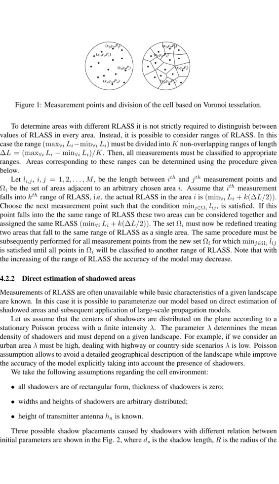
(xi, yi, Li),i = 1,2, . . . , M is insufficient for our purposes. Indeed, to estimateL andM we have to determine areas to which these measurements belong to. To determine areas with nearly the same RLASS we propose to use a division of the cell into areas whose vertexes are measurement points(xi, yi),i= 1,2, . . . , M.
In our case an appropriate division of the cell is given by Voronoi tesselation that separate a regionEof the spaceninto polygonsEi,i= 1,2, . . . , M, using a certain point process. In our case the space is2 and coordinates of measurement points can be considered as a realization of the point process on2. The polygonEi is the intersection of half planesTij bounded by the bisectors of the segments((xi, yi),(xj, yj)),i, j = 1,2, . . . , M and contain-ing(xi, yi)as a vertex. Practically, for each measurement point(xi, yi),i= 1,2, . . . , M,Ei, i= 1,2, . . . , M, is the area consisting of all locations in the space which are closer to(xi, yi)
than to any other measurement point. The system of all polygons forms a Voronoi tesselation. To ensure that the Voronoi tesselation is well defined the only requirement we impose on mea-surement points is that they must compose a non-degenerate realization of the point process. It means that there must be at least two measurement points, they are distinct, and there are only finitely many of these points in any bounded region. All these requirements are satisfied within our assumptions. There are a number of approaches to compute Voronoi tesselation (see [9] and references therein). An example of the division of the cell is shown in the Fig. 1.
(x1,y1,P1) (x2,y2,P2) (xi,yi,Pi) (xN,yN,PN) (x1,y1,P1) (x2,y2,P2) (xN,yN,PN) (xi,yi,Pi)
Figure 1: Measurement points and division of the cell based on Voronoi tesselation.
To determine areas with different RLASS it is not strictly required to distinguish between values of RLASS in every area. Instead, it is possible to consider ranges of RLASS. In this case the range(max∀iLi−min∀iLi)must be divided intoKnon-overlapping ranges of length ∆L= (max∀iLi−min∀iLi)/K. Then, all measurements must be classified to appropriate ranges. Areas corresponding to these ranges can be determined using the procedure given below.
Letli,j, i, j = 1,2, . . . , M, be the length between ithandjthmeasurement points and Ωi be the set of areas adjacent to an arbitrary chosen areai. Assume thatithmeasurement falls intokthrange of RLASS, i.e. the actual RLASS in the areaiis(min∀iLi+k(∆L/2)). Choose the next measurement point such that the condition minj∈Ωilij, is satisfied. If this point falls into the the same range of RLASS these two areas can be considered together and assigned the same RLASS(min∀iLi+k(∆L/2)). The setΩimust now be redefined treating two areas that fall to the same range of RLASS as a single area. The same procedure must be subsequently performed for all measurement points from the new setΩifor whichminj∈Ωilij is satisfied until all points inΩiwill be classified to another range of RLASS. Note that with the increasing of the range of RLASS the accuracy of the model may decrease.
4.2.2 Direct estimation of shadowed areas
Measurements of RLASS are often unavailable while basic characteristics of a given landscape are known. In this case it is possible to parameterize our model based on direct estimation of shadowed areas and subsequent application of large-scale propagation models.
Let us assume that the centers of shadowers are distributed on the plane according to a stationary Poisson process with a finite intensity λ. The parameterλ determines the mean density of shadowers and must depend on a given landscape. For example, if we consider an urban areaλmust be high, dealing with highway or country-side scenariosλis low. Poisson assumption allows to avoid a detailed geographical description of the landscape while improve the accuracy of the model explicitly taking into account the presence of shadowers.
We take the following assumptions regarding the cell environment:
• all shadowers are of rectangular form, thickness of shadowers is zero;
• widths and heights of shadowers are arbitrary distributed;
• height of transmitter antennahais known.
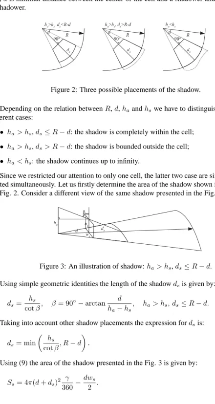
Three possible shadow placements caused by shadowers with different relation between initial parameters are shown in the Fig. 2, wheredsis the shadow length,Ris the radius of the
cell,dis minimal distance between the center of the cell and a shadower andhsis the height of shadower. 90o R 90o R R ha>hs, ds<R-d ha>hs, ds>R-d ha<hs ds ds ds 90o d d d
Figure 2: Three possible placements of the shadow.
Depending on the relation betweenR,d,haandhswe have to distinguish between three different cases:
• ha > hs,ds≤R−d: the shadow is completely within the cell;
• ha > hs,ds> R−d: the shadow is bounded outside the cell;
• ha < hs: the shadow continues up to infinity.
Since we restricted our attention to only one cell, the latter two case are similar and can be treated simultaneously. Let us firstly determine the area of the shadow shown in the left part of the Fig. 2. Consider a different view of the same shadow presented in the Fig. 3.
ha hs
ws b
ds d
Figure 3: An illustration of shadow:ha> hs,ds≤R−d. Using simple geometric identities the length of the shadowdsis given by:
ds= coths
β, β= 90
◦−arctan d
ha−hs, ha> hs, ds≤R−d. (8)
Taking into account other shadow placements the expression fordsis: ds= min hs cotβ, R−d . (9)
Using (9) the area of the shadow presented in the Fig. 3 is given by:
For those cases whenha > hs,ds> R−dorha< hsthe area is given by:
Ss= 4πR2360γ −dw2s. (11)
Finally, the area of the shadow can be expressed as: Ss= min 4πR2 γ 360,4π(d+ds)2 γ 360 −dw2s. (12)
The same estimation must be performed for all other shadowers obtained via realizations of the Poisson process and random variables describing widths and heights of shadowers. We have to note that the overlapping of shadows is also allowed. In this case the estimation of the shadows is still feasible.
To complete parametrization we have to estimate the RLASS valuesLi,i= 1,2, . . . , M, each of which is associated with appropriate area. To achieve it we propose to use classic large-scale propagation models. Most of these models assume that with the increasing of the distance between the transmitter and a receiverd, RLASS is decreasing according to a power law of dgiven a standard distanced0, whered0is often assumed to be1000meters for macrocells and100meters for microcells. For example, free space model assumes that there is only one unobstructed LOS path between the transmitter and a receiver and the mean propagation loss is given by [10]: E[L(d)] =Ls(d0) + 20 lg d d0 , (13)
However, it rarely occurs in practice that there is only one unobstructed propagation path between the transmitter and a receiver. Using measurements Okumura et. al. [1] obtained propagation curves for different environments. Hata [2] fits those data to empirical formulas and found that the mean propagation loss is proportional to separation distance as follows:
E[L(d)] =Ls(d0) + 10nlg d d0 , (14)
wherenis path loss exponent indicating the rate at which the pass loss increases with distance, d0is the standard distance,Ls(d0)is the propagation loss at the standard distance.Ls(d0)can
be measured or approximated [10].
If we take an assumption of free space propagation,n= 2and (14) degenerates to (13). If LOS is shadowedn >2. Considering urban areas, in certain circumstancesn <2(see [10] for a range ofnfor specific environments). Measurements carried out by Seidel et. al. [11] have shown that depending on a given propagation environment the actual propagation loss may deviate significantly from the mean given by (14). The actual value of propagation loss L(d)is log-normally distributed with meanE[L(d)]given by (14) and expressed as:
L(d) =Ls(d0) + 10nlg d d0 +Xσ, Xσ∈ {6−10}dB, (15)
transmitter and a receiver. Given a certain transmitted power, propagation loss can be related to RLASS [10].
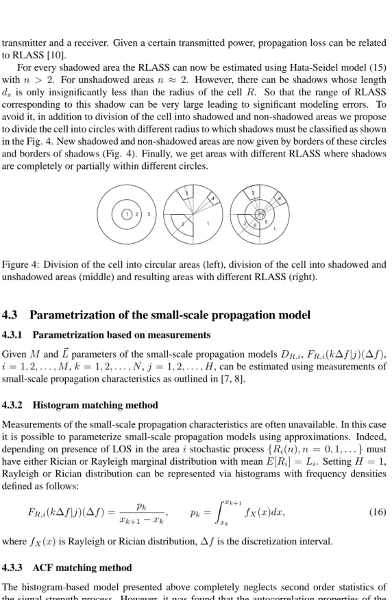
For every shadowed area the RLASS can now be estimated using Hata-Seidel model (15) withn > 2. For unshadowed areasn ≈ 2. However, there can be shadows whose length ds is only insignificantly less than the radius of the cell R. So that the range of RLASS
corresponding to this shadow can be very large leading to significant modeling errors. To avoid it, in addition to division of the cell into shadowed and non-shadowed areas we propose to divide the cell into circles with different radius to which shadows must be classified as shown in the Fig. 4. New shadowed and non-shadowed areas are now given by borders of these circles and borders of shadows (Fig. 4). Finally, we get areas with different RLASS where shadows are completely or partially within different circles.
7 6 1 2 3 2 3 4 1 2 3 4 1 5
Figure 4: Division of the cell into circular areas (left), division of the cell into shadowed and unshadowed areas (middle) and resulting areas with different RLASS (right).
4.3
Parametrization of the small-scale propagation model
4.3.1 Parametrization based on measurements
GivenM andL parameters of the small-scale propagation modelsDR,i,FR,i(k∆f|j)(∆f), i= 1,2, . . . , M,k= 1,2, . . . , N,j = 1,2, . . . , H, can be estimated using measurements of small-scale propagation characteristics as outlined in [7, 8].
4.3.2 Histogram matching method
Measurements of the small-scale propagation characteristics are often unavailable. In this case it is possible to parameterize small-scale propagation models using approximations. Indeed, depending on presence of LOS in the areaistochastic process{Ri(n), n = 0,1, . . .}must have either Rician or Rayleigh marginal distribution with meanE[Ri] =Li. SettingH = 1, Rayleigh or Rician distribution can be represented via histograms with frequency densities defined as follows: FR,i(k∆f|j)(∆f) = pk xk+1−xk, pk= xk+1 xk fX(x)dx, (16)
wherefX(x)is Rayleigh or Rician distribution,∆f is the discretization interval.
4.3.3 ACF matching method
The histogram-based model presented above completely neglects second order statistics of the signal strength process. However, it was found that the autocorrelation properties of the
received signal strength process influence the performance of wireless channels [8].
To provide more accurate model of the received signal strength in absence of statistical data we propose to set the lag-1 autocorrelation coefficient to a non-zero value:Ki(1)= 0.1Setting
H = 2the autocorrelation function (ACF)KR,i(n),n= 0,1, . . ., of{Ri(n), n= 0,1, . . .} is completely defined by the non-unit eigenvalueλ2,iofDR,i(λ1,i≡1). To approximate the autocorrelation properties of the received signal strength process we propose to minimize the approximation errorγby varying the values of(λ2,i, φi)according to the following expression:
γ= K
(1)−φ
iλ2,i
K(1) , λ2,i∈(0,1), (17)
whereφiis the variance of the{Ri(n), n= 0,1, . . .}.
To determine processes satisfying autocorrelation properties of the received signal strength process in the area we are given a triplet(E[Ri], φi, λ2,i), whereE[Ri] = Li. To determine
{Ri(n), n = 0,1, . . .}with a given triplet(E[Ri], φi, λ2,i)we have to set four parameters (G1,i, G2,i, dR,i,12, dR,i,21), whereG1,i and G2,i are mean signal strengths in the states 1 and 2 respectively, dR,i,12 is the transition probability from state 1 to state 2,dR,i,21 is the transition probability from state 2 to state 1 of{SR,i(n), n = 0,1, . . .}. If we chooseG1,i such thatG1,i < E[Ri]to satisfy0 < λ2,i <1we can obtainG2,i,dR,i,12anddR,i,21from the next set of equations:
⎧ ⎪ ⎪ ⎨ ⎪ ⎪ ⎩ G2,i= E[Ri]φ−G1,i +G1,i dR,i,12=(1−λ2G)(2,iE−[RGi1]−,iG1,i) dR,i,21=(1−λ2G)(2,iG−2,iG−1,iE[Ri]) . (18)
It is clear from (18) that there is a degree of freedom choosing the value ofG1,i. Thus, there are infinite number of processes with the same triplet (E[Ri], φi, λ2,i). As a result, the abovementioned derivation restricts us to RLASS, variance and ACF and does not cap-ture distribution of the received signal strength process. Since the stationary probabilities of
{SR,i(n), n = 0,1, . . .} can now be found, for frequency densities of Rayleigh or Rician
distribution the next equations holds:
⎧ ⎪ ⎨ ⎪ ⎩ 2 i=1FR,i(k∆f|j)(∆f)πR,i,j = xk+1pk−xk k= 1,2, . . . , N N j=1FR,i(k∆f|j)(∆f)k∆f =Gi,j j= 1,2 N j=1FR,i(k∆f|j)(∆f) = 1 j= 1,2 , (19)
whereπR,i,j,j = 1,2are the stationary probabilities of{SR,i(n), n= 0,1, . . .},pk is the frequency density,Gi,jis the mean received signal strength in the statej,j= 1,2.
Note that in (19) we have only(4 +N)equations and2Nunknowns. To determine values ofFR,i(k∆f|j)(∆f),k= 1,2, . . . , N,j = 1,2, we propose to use the random search algo-rithm. According to it we must choose a required approximation error of the signal strength distribution and then assignFR,i(k∆f|j)(∆f),k = 1,2, . . . , N,j = 1,2, such that (19) is satisfied. The algorithm is outlined in details in [12].
1Actually, the value ofK
5
Conclusions
In this paper we presented an extension to existing wireless channel modeling techniques ex-plicitly taking into account the movement of the user between areas with different small-scale propagation characteristics. The proposed model has straightforward applications in perfor-mance evaluation of IP-based applications in presence of signal changes caused by movement of the user between areas with different propagation characteristics.
References
[1] T. Okumura, E. Omori, and Fakuda K. Field strength and its variability in VHF and UHF land mobile service. Review of electrical communication laboratory, 16(9/10):825–873, September/October 1968.
[2] M. Hata. Empirical formula for propagation loss in land mobile radio services. IEEE Trans. on Veh. Tech., VT-29(3):317–325, August 1980.
[3] J. Andersen, T. Rappaport, and S. Yoshida. Propagation measurements and models for wireless communications channels. IEEE Comm. Mag., 33:42–49, Nov. 1995.
[4] S. Seidel and T. Rappaport. Site-specific propagation prediction for wireless in-building personal communication system design. IEEE Trans. on Veh. Tech., 43(4):879–891, November 1994.
[5] A. Saleh and R. Valenzuela. A statistical model for indoor multipath propagation. IEEE JSAC, 5(2):128–137, February 1987.
[6] D. Durgin and T. Rappaport. Theory of multipath shape factors for small-scale fading wireless channels. IEEE Trans. on Ant. and Propag., 48:682–693, May 2000.
[7] Q. Zhang and S. Kassam. Finite-state markov model for Rayleigh fading channels. IEEE Trans. on Comm., 47(11):1688–1692, November 1999.
[8] J. Swarts and H. Ferreira. On the evaluation and application of markov channel models in wireless communications. In Proc. VTC’99, pages 117–121, 1999.
[9] P. Green and R. Sibson. Computing dirichlet tesselations in the plane. Computer Journal, 21:168–173, 1978.
[10] T. Rappaport. Wireless communications: principles and practice. Communications en-gineering and emerging technologies. Prentice Hall, 2nd edition, 2002.
[11] S. Seidel. Path loss, scattering and multipath delay statistics in four european cities of digital cellular and microcellular radiotelephone. IEEE Trans. on Veh. Tech., 40(4):721– 730, November 1991.
[12] D. Moltchanov, Y. Koucheryavy, and J. Harju. The model of single smoothed MPEG traffic source based on the D-BMAP arrival process with limited state space. In Proc. of ICACT, pages 55–60, Phoenix Park, S. Korea, January 2003.