Most Stringent Test for Location Parameter of a Random Number from Cauchy Density

Munich Personal RePEc Archive

Most Stringent Test for Location

Parameter of a Random Number from

Cauchy Density

Atiq-ur-Rehman, Atiq-ur-Rehman and Zaman, Asad

IIIE, international islamic university, islamabad

March 2008

Online at

https://mpra.ub.uni-muenchen.de/13492/

Email:

International Institute of Islamic Economics International Islamic University, Islamabad

E mail:

International Institute of Islamic Economics International Islamic University, Islamabad

α θ

____________

1.

Introduction

Cauchy Distribution (or Lorentz Distribution in terminology of Physicists) has its applications in Physics, Spectroscopy and in Statistics. It is used to measure the sensitivity of an estimator\test statistics to normality assumptions due to its heavier tails which are extremely unlikely under normality assumptions.

Since the moments are not defined for Cauchy distribution, the tests/estimators based on asymptotic properties are not appropriate while studying the properties of Cauchy distributions. Statistician had discussed some statistical properties of the distribution. The principal focus of studies is on goodness of fit to the Cauchy distribution. The studies of Rublyk (1997), Rublyk (1999) Gurtler & Henze (2000), Rublyk (2001), Rublyk (2003) and Matsui & Takemura (2005) are the examples. Other studies explore parameter estimation, & behavior of Likelihood function etc. See Copas (1975), Besbeas & Morgan (2001) and Lawless (1972) for example.

For an observation X from Cauchy distribution, we explore the tests for location parameter of the distribution with focus on point optimal (Neyman Pearson) tests & develop method to find out the most stringent test. Lehman (1986) discussed that for location parameter of an observation X from Cauchy density, UMP test does not exist. Obviously the Stringent test is the feasible choice in absence of UMP test if we can find it. We study the power properties of a large number of NP1 tests and develop technique to find out power envelop and power curve of a point optimal test of given size, and hence to find shortcoming of test. By luck of draw, the problem turned to be different in its nature, in that, we are able to construct the power envelope analytically. Similarly we can trace power curves of a point optimal test as well. This made possible the computation of shortcoming of a large number of point optimal tests. The techniques are discussed below.

___________________________________

1

2.

The problem

Let Ca(θ) denotes the Cauchy distribution, with location parameter θ and unit scale parameter & X ~ Ca(θ) i.e.

f(X|θ) =

1

π1+

(

)

We are interested in testing the Hypothesis H0: θ = 0 versus H1: θ > 0. The Null space Θ0

= (0) and the alternative space Θ1 = R+.

3.

Point Optimal Test & Power Envelope

3.1

Test Statistics for Point Optimal Test & Critical Values

Given the problem, Neyman Pearson Lemma allows us to construct test optimal for a point θ ∈Θ1. Let L(X,θ ) denote density at X given the location parameter θ than

the test statistics is:

L X 0

(

)

(

)

For test of size α the critical values can be computed by assuming H0 is true &

finding Cα(θ) such that

P L X

(

)

L X 0( , ) ≥Cα

( )



  α

[1]

Where P(.) denotes probability & the subscript α refers to size of the test. Now For Cauchy density,

L X

(

)

π1+

(

)

 −1

π

(

)

 −1

1+ X2

Given an observation X, we reject the null if L(X,0,θ) > Cα(θ) and accept

otherwise. This procedure maximizes power at θ ∈Θ1. By changing θ, we get different

test statistics optimizing power for that new point.

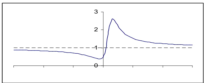
Now, for θ ∈ Θ1, we plot L(X,0,θ) for different values of X. A Typical graph is

shown in fig 1.

Fig 1: A Typical Plot of L(X,0,θ)

The solid line denotes the values of L(X, 0,θ). The graph cuts the line y =1 (the dotted line) at one point and converges to 1 as X converges to ± ∞

The graph of L(X,0,θ) is increasing in a finite interval and decreasing otherwise. L(X,0,θ) = 1 only at X= θ/2. Little mathematical formulation verifies that for X>θ/2, L(X,0,θ) is greater than 1 & smaller than 1 otherwise. For finite θ, the graph of L(X,0,θ) converges to 1 if X → ±∞.

Below we discuss how to find out the critical value Cα(θ) analytically.

C_α

( )

2

+ +4θ2k

(

)

2

4 4

(

)

− +

2 4

(

)

Where Cα(θ) be defined in [1] above and

k tan2

( )

Using definition of Cα(θ),given size of test = α & assuming H0 is true, Cα(θ) is the value

such that

P L X

(

)

L X 0( , ) ≥Cα

( )



  α

[2]

To find Cα(θ), solving the equation,

1+ X2

1+

(

)

Cα

( )

[3a]

For simplicity, denote Cα(θ) by C, we can rewrite [3a] as:

X2(1−C)+2CXθ+1−C−Cθ2 0. [3c]

Supposing l, m being the roots of equation [3b], since l, m specify the range where we reject the Null. So assuming the Null is true, integration of the density function over range (l, m) must be equal to size of test α i.e.

1

π

(

)

⌠   ⌡

α

⇒ 1

π

1

−

( )− −1( )

  α

⇒ −

1+

( )

[3c]

Now l, m being roots of equation [3b] quadratic in X, therefore:

+ −2 "θ 1−"

1−"−"θ2

1−"

[3e]

Solving [3c], [3d], and [3e] for C yield:

8⋅"+4⋅"2⋅θ2−4−4⋅"

2−2⋅"−"θ2

(

)

2

( )

Assuming 2

( )

And solving [4] for C gives:

(

)

(

)

2 4 2 2 2 2 2 4 4 4 2 ) 4 4 )( 4 4 4 ( 4 4 4 8 8 4 4 8 8

θ

θ

θ

θ

θ

θ

θ

θ

This equation gives two values of C corresponding to

θ α and θ α

Obviously we are interested in first expression, for that we have to choose the larger root of C. i.e.

(

)

(

)

2 4 2 2 2 2 2 4 4 4 2 ) 4 4 )( 4 4 4 ( 4 4 4 8 8 4 4 8 8

θ

θ

θ

θ

θ

θ

θ

θ

Replacing C by Cα(θ), yield proof of theorem.

We completely specify our test statistics and the critical values to be used throughout in the discussion of Neyman Pearson tests as:

Test Statistics: L(X,0,θ) = ( 1+X2 )/( 1+(X θ)2 )

Critical Value: Cα(θ) (defined & derived in theorem 1)

The test statistics and the critical values vary with the variation of θ.

3.2 Critical value & the power properties

It was observed that power of an NP test depends crucially on Cα(θ). The

relationship of power of a test and the critical value Cα(θ) is discussed in the following

For convenience, let θ denote the point at which we are maximizing power & β be the point in R+ for which we want to compute the power of a test. Further Tθ denote NP test optimal for θ∈ R+. Than for an NP test;

1. If Cα(θ) >1, power of Tθ converges to zero for the large β.

2. If Cα(θ) ≤1, power of Tθ converges to 1 for the large β.

Proof:

Remember we reject the null if L(X,0,θ) > Cα(θ)

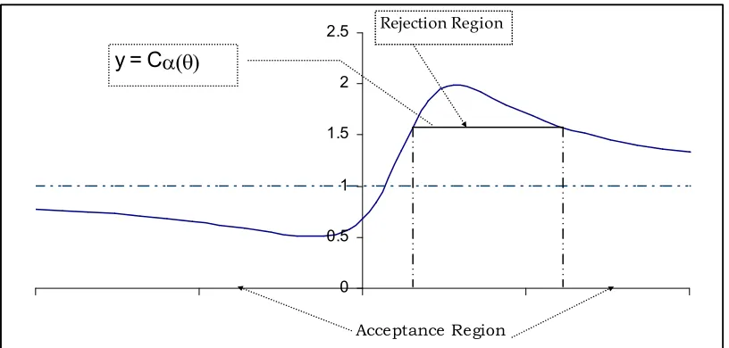
a) If Cα(θ) >1, than roots of equation [3b] lies on RHS of point X=θ/2. Let be

the roots of quadratic equation [3b], than the roots determine boundaries of rejection region. It can be shown unique maxima of L(X,0,θ) lies inside interval ( ). Therefore the rejection region is bounded by roots . Than for some θ∈ R+, power of test is just integration of density function f(X|β) on interval ( ).

Fig 2: Rejection region when Cα(θ) >1

α(θ)

Value of L(X,0,θ) is large than Cα(θ) for points between root of L(X,0,θ) = Cα(θ) which is the rejection region

∞

β $

θ_,β

(

)

→ = β ∞

1 π1+

(

)

⌠   ⌡

→

=

∞ β

1 π

1

−

(

)

(

)

(

)

 .

→

= 0

b) We divide proof of [b] in to two parts

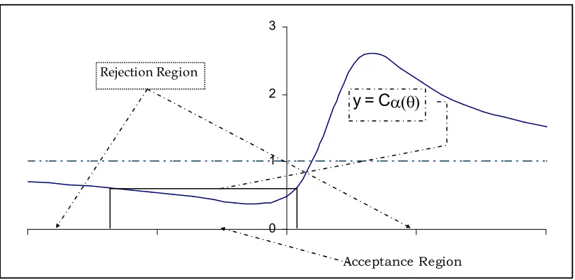
i) If Cα(θ) <1, than roots of equation [3b] lies on left of point X=θ/2.

Again if be the roots of quadratic equation [3b], they determine boundaries of rejection region. It can be shown unique minima of L(X,0,θ) lies inside interval ( ). Therefore the rejection region is R ( ). Therefore for some β ∈ R+, power of test is integration of density function f(X|β) on real line minus integration of density function on interval ( ).

Fig 3: Rejection region when Cα(θ) <1

α(θ)

Value of L(X,0,θ) is smaller than Cα(θ) for points between root of L(X,0,θ) = Cα(θ) which is the acceptance

region

∞ β

$θ,β

(

)

→ = β ∞ 1 !

1

π1+

(

)

⌠   ⌡ −       →

= 1

∞ β 1 π 1 −

(

)

(

)

(

)

 .

→

− = 1

ii) If Cα(θ) =1, than we are just at X=θ/2and as we had discussed, for all

points on right side of θ/2, L(X,0,θ) >1. The two roots of quadratic equation [3b] are θ/2 and ∞. So power of such test for a β ∈ R+ is integration of density function f(X|β) on range (θ/2, ∞). Finding probability of accepting Null for large β;

∞ β

1−R T

(

)

(

)

⌠   ⌡ → = ∞ β , 1 π 1 − θ

2 −β



 

1

−

₍

₎

− 

 

→ = 0

Since probability of accepting Null for large β is 0, the power of test will be 1.

Theorem 2 realizes the important role of the critical value in determining the power properties of a test. If the critical value is larger than 1, the test is sure to have zero power for the large alternatives. Whereas the test with critical value smaller than 1 has 100% power for the same alternatives. Therefore the former tests with critical value larger than 1 are sure to have 100% shortcoming & should never be used in absence of precise prior information of the alternative.

3.3

Power Envelope

For a test optimal at point θ∈Θ1 we discussed how we can find power of the test

forms the power envelope. The algorithm to trace power envelope is discussed in greater detail in appendix.

4.

Performance of Conventional NP tests

Up to best of our knowledge, none of existing studies had addressed the problem we are discussing. However in general hypothesis testing problems, when there is no UMP test, different strategies had been recommended in the Literature to design a feasible NP test. Below we discuss the some of the strategies & their performance in the present problem. We discuss three types of conventional hypothesis testing strategies:

A) Maximizing power in neighborhood of Null (the Locally Most Powerful or LMP tests)

B) Maximizing power for extremely large alternatives (Berenblutt & Webb Type tests)

C) Maximizing power for some intermediate choice of alternatives

4.1

The Locally Most Powerful test

The rational of a Locally Most Powerful test (LMP) is to maximize power for an alternative in the neighborhood of Null. Choice of an LMP test for testing location parameter in the problem discussed turned out to be most unsuitable as the LMP test possess 100% shortcoming. It turns out that for an LMP, Cα(θ) >1, therefore according to

theorem 2, the test has zero power for the large alternatives. Whereas, as we will show later, there is a certain class of test for which Cα(θ) <1 & hence possess 100% power for

large alternatives. Therefore the LMP test has 100% shortcoming. The following Lemma proves the claim.

Proof:

We can rewrite expression for Cα(θ) derived in theorem 1 as:

Cα

( )

2

+ + 4θ2k+ 4θ (1+k) 2

(

)

2 4

(

)

[6]

Let θ be so small that it higher powers are negligible than the expression reduces to:

Cα

( )

2 4( + 4 k⋅ )

[6b]

Obviously, for θ > 0 the numerator of expression on right hand side of [6b] is greater than denominator. Hence Cα(θ)>1.

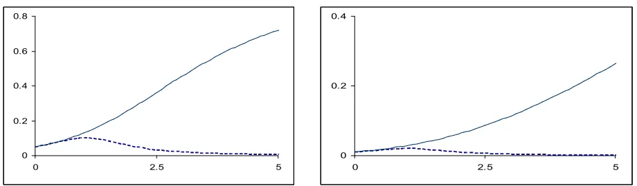
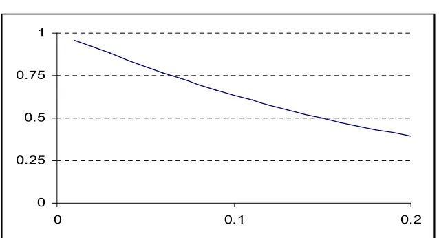
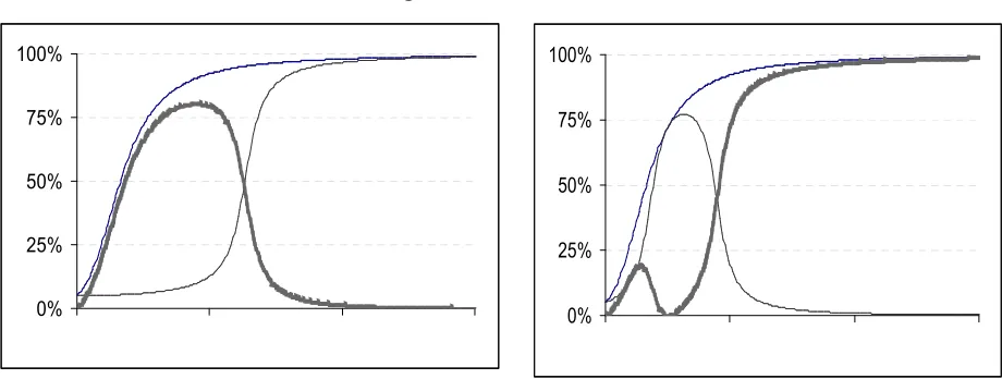
The Lemma gives crucial information about the power curve of LMP test, in that, the critical value of LMP is larger than 1 & thus according to theorem 2, have zero power for large alternatives. Therefore, LMP has 100% shortcoming. So LMP should never be used if we don’t have precise information of θ. Empirical results shows that LMP is not good even outside a small neighborhood of the point for which it is optimal. A test of size 5% optimal for θ = 0.5 has only 1% power for θ = 4 and for θ = 15, its power is zero up to 3 decimal places.

Fig 4: Performance of LMP test

The solid lines in the two graphs represent the power envelope whereas the dotted lines represent power curves of test optimal for θ = 0.1. Size of test is 5% for the left panel and 1% for the right panel. Immediate decline in power of LMP is obvious in the

So having no prior information of the true parameter, the choice of LMP test is hazardous.

4.2

Berenblutt & Webb type test

In their discussions of tests for autocorrelation, Berenblutt & Webb (1973) recommend to use another extreme strategy, to maximize power for largest possible alternative. The alternative space we have is R+ ranging from 0 to ∞, therefore we have maximize power for ∞ . One of the result of following Lemma is the proof that; β → ∞

⇒ Cα(θ) → 0 < 1, and thus (by theorem 2) the test has 100% power for large

alternatives.

Lemma 2:

For Cα(θ) defined in [2], following results hold.

R1 _{β ∞} "α

( )

→

R2 _{β ∞} "α

( )

→

R3

∞

β "α

( )

2

⋅ 2+ 2⋅ 2 (1+ ) 2 θ

2 +

(

)

Where ‘k’ is defined in [4b] above. Proof:

Again for simplicity, denote Cα(θ) by C than for R1

∞

β→ "α

( )

∞ θ

8+8 + 4θ2+4θ2 + 4θ (1+ ) 2

(

)

2 4

(

)

→

=

∞ θ

8+8⋅ +4⋅θ2+4⋅ ⋅θ2

θ4

4⋅θ⋅ (1+ ) 2⋅

(

)

θ4

+

2 4+4⋅ θ

4

+ + 4⋅ θ2

(

)

θ4

⋅

→

= 0

Similarly for R2

∞ β

"_α

( )

→ = _{θ ∞}

8θ +8 k⋅ θ+4⋅θ3+4⋅θ3⋅k

θ4

4⋅θ2⋅ (1+k) 2⋅

(

)

θ4

+

2 4+4 k⋅ kθ

4

+ + 4 k⋅ θ2

(

)

θ4 ⋅

lim

→

= 0

And for R3:

∞

β "α

( )

2

→ =

∞ θ

8θ2+ 8⋅ θ2+4⋅θ4+4⋅ ⋅θ4

θ4

4⋅θ3⋅ (1+ ) 2⋅

(

)

θ4

+

2 4+ 4⋅ θ

4

+ +4⋅ θ2

(

)

θ4

⋅

→

= 2+ 2 +2 1+

Hence the results

Solving equation [3] for X & using results of Lemma 2, one can find out the range for which B&W type test rejects Null. It is observed that power curve of B&W type test is increasing in β. So, obviously the tests of this type are preferable to LMP in that they have smaller shortcoming than LMP.

Fig 5: Shortcoming of B&W type tests

Size of test represented on X axis & shortcoming of B&W on Y axis. Shortcoming of B&W type test is less than 1, but still massive

For size 1%, the test has 96% shortcoming, which is obviously disappointing, and for size 20%, the shortcoming is 40%. That is, we still have a lot of loss in using this type of test. As we will soon show, there is an intermediate class of tests other than B&W type tests, all of which has 100% power for infinitely large alternatives. Is it possible to choose a test in that class which has smaller shortcoming? Next we investigate the same question.

4.3 Intermediate choice of Alternative

Cases where both LMP and B&W type tests perform poorly, it is natural to choose an intermediate alternative to optimize power for. Several strategies are recommended by different writers to choose a suitable intermediate. See Efron (1975), Davies (1969) Fraser et al (1976) & King (1985) for example.

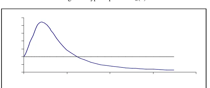
Fig 6: A typical plot of Cα(θ)

Cα(θ) is large than 1 for a finite range and than decreases continuously

We see that for test of fixed size, there exist a θm∈ R+ with Cα(θ) = 1 and

Cα(θ) >1 θ∈ ( 0, θm)

Cα(θ) <1 θ∈ ( θm , ∞)

Now if we choose an alternative in ( 0, θm), Cα(θ) >1, an NP test optimal in this interval

is the test with maximum shortcoming. Whereas for choice of θ ∈ ( θm , ∞) the test is certain to have 100% and power for very large alternative. Now first step in an analysis is to search θm so that we can avoid choosing a test with 100% shortcoming.

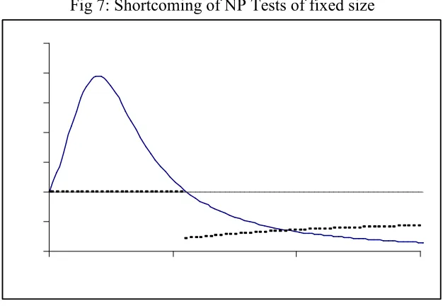
Luckily, we are able to compute critical value of an NP test analytically as well as we can analytically compute power of an of NP test at any point. This makes computation of exact power envelope, power curve & shortcoming of a test possible. We compute the shortcoming of a large number of NP tests. E.g. for size of test > 5% we compute shortcoming of test optimizing power at each point of the vector (0, 0.5…10000) to choose a feasible alternative which minimizes the shortcoming (The algorithm given appendix). We found that for the test optimal for θm (θm defined above), shortcoming is

Fig 7: Shortcoming of NP Tests of fixed size

Dotted line indicates shortcoming of the test, whereas the solid line is for value of Cα(θ). Shortcoming suddenly drops

down for Cα(θ) = 1 and then increases monotonically with θ

Tests optimal for any point in ( 0, θm) have 100% shortcoming, which is according to our

expectation. Than shortcoming suddenly drops down for Tθm and than increases monotonically with θ and converges to shortcoming of B& W type tests. The pattern of plot remains same for different size of test.

There are some other strategies to choose a feasible alternative, e.g. using the information matrix etc. But in our case, any strategy for choosing a feasible intermediate point optimal test falls into one of the two categories discussed & therefore there is no need to study them separately.

5.

Recommended test

search for a point θm in R+ such that Cα(θm) = 1. Having an analytical formula to

compute Cα(θ), this is worth spending few moments on computer. In table 1, we tabulate

θm for different sizes. It was observed that Tθm has significantly smaller shortcoming than

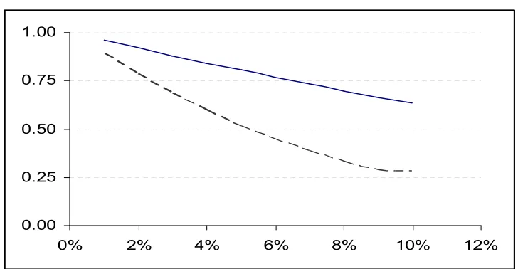
that of B&W. Below we plot the shortcoming of the two types (Tθm and B&W) of test for size 1 10%.

Fig 8: Comparison of Tθm and B&W test

Dotted line represent shortcoming of Tθm which is much smaller than shortcoming of B&W type test represented by solid line.

5.1 Other Characteristic of Recommended Test

θθθθ

It can be seen from fig 8 that shortcoming of Tθm increases by a large factor if we reduce size of test by 1%. Reducing size of test from 5% to 4% increases the shortcoming from 51% to 59%. Hence the arbitrary choice of size of test is risky. It’s better to choose the larger size since it cuts down shortcoming by multiple factor.

θθθθ _!

the alternative is some β ≠θm. So, one may think to use an NP test optimal for β to get a

larger power. There are two possibilities

If β < θm than using Tβ may be beneficial by a large amount in the neighborhood of β but

as we had discussed, the test may have zero power if the true parameter is larger than our belief. We are at risk of 100% shortcoming.

If β > θm than surprisingly, Tβ is not much beneficial even in the neighborhood of β. We

computed the maximum shortcoming of Tθm of different sizes on the range (θm, ∞) which

is tabulated below. It turns out that the maximum difference between power envelope & power curve of Tθm is negligible in interval (θm, ∞).

"

Size of test θm SC of Tθm on (θm, ∞)

1% 63.642 0.0009

2% 31.790 0.0018

3% 21.158 0.0027

4% 15.832 0.0036

5% 12.628 0.0045

6% 10.485 0.0054

7% 8.948 0.0063

8% 7.790 0.0072

9% 6.885 0.0081

10% 6.156 0.0091

For test of any size, the maximum advantage we can have to maximize power beyond θm

Figure 9: Abuse of Tθm

Solid lines in the two graphs represent power envelope and lines with dashed lines represent power curves of Tθm. The Dotted line in left panel represent power curve of an NP test optimal in (0, θm). The test has significant gain over Tθm for a small range,

but zero power for large alternatives. In right panel, dotted line denote point wise shortcoming of Tθm which is negligible for range (θm, ∞) Whereas, optimizing beyond θm will always increase shortcoming. Optimal choice in this case is again Tθm.

Solid lines in the two graphs represent power envelope and lines with cross marks represent power curves of Tθm. The Dotted line in left panel represent power curve of an NP test optimal in (0, θm). The test has significant gain over Tθm for a small rang, but zero

power for large alternatives. In right panel, dotted line denote point wise shortcoming of Tθm which is negligible for range (θm, ∞).

Whereas, optimizing beyond θm will always increase shortcoming. Optimal choice in this

case is again Tθm.

#

"

The first author likes to acknowledge the contribution of Higher Education Commission of Pakistan, which is sponsoring him for higher education through indigenous fellowship scheme.

6. Appendix

Suppose we want to trace power curve of a test of size α which optimizes power at θ ∈ R+. A lot of computational burden is released by the analytic formula in our hands. Even without computing the actual test statistics, we can compute the critical value by the formula derived in theorem1. Putting the critical value in [3b] and solving for X, yield the roots . Theorem 2 allows us to specify the range for which value of actual test statistics will be larger than critical value. That is if critical value ‘Cα(θ) ’ is larger than 1,

the rejection region is bounded by the roots i.e. L(X,0,θ) > Cα(θ) if < X <

Now to compute power of test for some θ ∈ R+, the power of test is probability that random variable X lies in specified range.

∞

β $

θ_,β

(

)

→ =

P [ ≤ X ≤ ]

= _π 1

1+

(

)

 

⌠   ⌡

Now once we have specified range for which null should be rejected for Tθ, The locus of R(T, β), gives the power curve. The power curves discussed in paper were traced by computing power at β = 0, 0.5 …10000 for size of test > 5% and at β = 0, 1…50000 for size of test < 5%. Computing R(Tβ , β) yield power envelop for β = 0, 0.5…10000. For any test T, R(Tβ , β) R(Tθ, β), β = 0, 0.5 …10000 yield vector of point wise shortcoming, and maximum of this vector is the shortcoming of the test.

6.2 References

[1] Berenblutt I. & Webb G.I. (1973) ‘A new test for autocorrelated errors in linear regression model’ Journal of Royal Statistical Society, series B34

[2] Copas J.B (1975). ‘On Unimodality of the Likelihood for Cauchy distribution’ Biometrika, 62

[4] Efron B. ‘Defining curvature of a statistical problem’ Anals of statistics, 3(6)

[5] Fraser D.A.S. Guttman I. & Styan G.P.H. (1976), ‘Serial correlation and distribution on a sphere’ Communications in Statistics

[6] King M.L. (1987) ‘Toward a theory of point optimal testing’ Econometric Reviews

[7] Gurtler N. & Henze, N. (2000). ‘Goodness of fit tests for Cauchy distribution based on the empirical characteristic function’ Ann. Inst. Statist. Math, 52

[8] Lawless J. F. (1972). ‘Conditional confidence interval procedure for location & scale parameters of the Cauchy and logistic distribution’ Biometrika, 52

[9] Lehman E.L. (1986). ‘Testing Statistical Hypothesis’, 2nd Edition, John Wiley & Sons, Inc

[10] Matsui M. & Takemura A.(2003). ‘Empirical Characteristic Function Approach to Goodness of Fit Test for Cauchy Distribution with Parameters estimated by MLE or EISE’ CIRJE discussion paper series, University of Tokyo

[11] Rublyk F. (1999). ‘A goodness of fit test for Cauchy distribution’, Proceedings of the Third International Conference on Mathematical Statistics, Tatra Mountains, Mathematical Publications Bratislava

[12] Rublyk F. (2001) ‘A quantile goodness of fit for Cauchy distribution, based on extreme order statistics’. Applications of Mathematics