Identifying good inflation forecaster

Munich Personal RePEc Archive

Identifying good inflation forecaster

Duasa, Jarita and Ahmad, Nursilah

2008

IDENTIFYING GOOD INFLATION FORECASTER

Jarita Duasa Nursilah Ahmad

Abstract

The objective of this paper is to identify the best indicator variable in forecasting inflation in Malaysia. Due to the fact that Malaysia experienced the rise of CPI by 4.8 percent in March 2006, the country’s highest inflation rate in seven years, there is a need to foresee future trend of general price level. To determine whether certain indicator (variable) could predict inflation, we construct a simple forecasting model that incorporates the variable. We estimate a two-variable VECM model of quasi-tradable inflation using monthly data covering the period 1980:01 to 2006:12. We alternate between the following inflation indicators: commodity prices, financial indicators and economic activities. We evaluate each model using out-of-sample forecast. The study proposes that a simple model using industrial production index improves the accuracy of inflation forecasts. The results support our hypothesis.

Keywords: goods inflation; VECM ; Malaysian economy.

High inflation is one of important macroeconomic problems which need to be curbed by authority in any economy. In designing appropriate policy measures for inflation problem, policy makers need to forecasts of inflation. A period often used for policy discussion in forecasting inflation is 24-month horizon. The issue here is what indicator could best used to forecast actual inflation.

There is a debate on what variable should be used to better forecast inflation. The literature suggests various indicators such as commodity prices, financial indicators or economic measures; either in level or growth forms. We attempt to investigate which inflation indicators best predict future inflation Furthermore, we test whether one of these indicators individually improve the forecast of inflation. The evaluation is based on root-mean-squared-error (RMSE) statistics. We follow Stock and Watson (1999) and Cechetti et al. (2000) method in our estimation.

This paper is organized as follows. The next section gives an overview of inflation trend in Malaysia. In Section 3, we outline statistical properties of the data and model specifications. Section 4 discusses the results. Section 5 concludes.

2. Inflation Trend in Malaysia

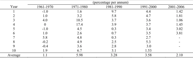
Over the past decades, the inflation rate in Malaysia has been relatively volatile. Beginning with a low averaged level of 1.1 percent over 1961-1971, the inflation rate increased and peaked at unprecedented high level of 17.4 percent in 1974 and again at 9.7 percent in 1981. While for the most years of 1980s, the rate of inflation is relatively low and steadily decreasing, it started rising again in 1988 (Ibrahim, 1996). In March 2006, CPI rose by 4.8 percent, marking the country’s highest inflation rate in seven years. Table 1 summarizes growth in CPI over the period 1961-2006.

Table 1: Growth in CPI, 1961-2006

(percentage per annum)

Year 1961-1970 1971-1980 1981-1990 1991-2000 2001-2006

1 -1.0 1.6 9.7 4.4 1.42

2 1.0 3.2 5.8 4.7 1.81

3 4.0 10.5 3.7 3.6 1.06

4 0 17.4 3.9 3.7 1.45

5 -1.0 4.5 0.3 3.4 3.02

6 1.0 2.6 0.7 3.5 3.81

7 5.8 4.8 0.3 2.7 -

8 -0.2 4.9 2.5 5.3 - 9

10

-0.4 1.9

3.6 6.7

2.8 3.1

3.0 1.53

-

Average 1.1 5.98 3.28 3.58 2.10

Source: BNM, 1999 and IFS CD ROM, 2006.

thereafter. Unemployment seems to remain quite stable but inflation is on the rise since 2004.

Figure 1: Inflation and Unemployment in Malaysia, 1984-2006

0 1 2 3 4 5 6 7 8 9 198 4 198 5 198 6 198 7 198 8 198 9 199 0 199 1 199 2 199 3 199 4 199 5 199 6 199 7 199 8 199 9 200 0 200 1 200 2 200 3 200 4 200 5 200 6 unemployment CPI

Source: BNM, 1999 and IFS CD ROM, 2006.

For the period of 1970s, inflation rate in Malaysia “was primarily imported” (Semudram, 1982, 1987; Rana, 1984). That is, the external sources of inflation (measured by percentage change in import price index or the percentage change in foreign inflation rate and in import-weighted exchange rate) are found to have large and significant impact on Malaysian inflation rate. Meanwhile, Tan and Cheng (1995) conclude that money causes inflation in Malaysia. In other words, inflation is a monetary phenomenon. Thus, inflationary behaviour in Malaysia is the consequence of both internal and external factors (Ibrahim, 1996).

Domestically, inflationary pressures continue to be present, partly due to the rising oil prices. Given this cyclical behaviour of inflation rate, getting an accurate, reliable and consistent forecast of inflation is important. This is highly relevant since inflation stability is one of the Bank Negara’s main objectives.

3. Method

Cechetti et al. (2000) discuss three broad classes of inflation indicators. First, commodity prices such as specific prices for oil or indexes of a group of such goods. Second are the financial indicators such as exchange rates and monetary aggregates. Third are indicators of the status of the real economy. Capacity utilization, and unemployment rates are often regarded as variables that presage change in the CPI.

In this study we use the following indicators: CPI to denote quasi tradable CPI;

ALLCPI to denotes unadjusted CPI and used as the upper boundary; oil prices, OIL

represent commodity price; money supply, MI to represent financial indicator and; industrial production index, IPI as an economic measurement. The variables used are listed in Table 2 below.

Variables Descriptions Sources

CPI Consumer price index, a measure for inflation This is “quasi-tradable” CPI measurement which comprises all goods

IFS CD-ROM April , 2007

ALLCPI OIL

Unadjusted CPI

World oil price in US dollar and proxied by West Texas Intermediate

BNM publications

IFS CD-ROM April , 2007

MI Money supply M1 as a measure of financial indicator

IFS CD-ROM April , 2007

IPI Industrial production index as a proxy for aggregate demand

IFS CD-ROM April , 2007

OIL is denoted in US dollar per barrel to indicate that it is exogenous to the economy. This is the monthly price of West Texas intermediate average crude price of petroleum deflated by CPI all items city-average of the United States (2000=100). We do not use domestic currency because the fluctuations of local currency oil prices for East Asian countries from the mid 1990s largely reflects not the oil price per se but the variability of bilateral exchange rate vis-à-vis the US dollar (Ito et al., 2005). MI is the money supply. IPI is the proxy for the economic activities.

Unlike Cecchetti et al. (2000), this study applies vector error correction model (VECM). We use a set of p=2 endogamous variables, y = [cpi, ind]` where cpi and ind refer to the logarithm of CPI and IND is the specific indicator variable, respectively. We write a p-dimensional vector error correction model (VECM) as follows:

_{t i t t}, t = 1, . . .T

k i

i

t y y

y = ΓΔ +Π +μ+ε

Δ

∑

where y_t is the set of I(1) variables discuss above; ε_t~niid(0,∑); μ is a drift parameter, and Π is a (p x p) matrix of the form Π=αβ′where αand βare both (p x r) matrices of full rank, with β containing the r cointegrating vectors and α carrying the corresponding loadings in each of the r vectors. We include monthly dummy and financial crisis dummy, DUM01 in which 0 is assigned to the period before June 1997 and 1 otherwise.

We estimate the model using data from 1980 through the end of 1990 to produce inflation forecast for 1991-1992 period. Next, we re-estimate the model using data through the end of 1992 to forecast inflation for 1993-1994 period, data through the end of 1994 to predict inflation for 1995-1996 period, and so forth. This procedure enables us to track the performance of indicators in different years to assess the robustness of their predictive power.

To assess the accuracy and reliability of inflation forecast, we use RMSE statistics, following Cecchetti et al. (2000). This statistics measures the degree to which the predicted change in the CPI deviates from the actual change from the forecast period. The indicator variable’s ability to forecast inflation is determined if the variable, when added to the model, lowers the RMSE.

an indicator as independent of inflation if inflation does not granger-cause the indicator.

3.1 Data and Variables

We use the “quasi-tradable” CPI (hereafter CPI) measurement which comprises all goods following Obstfeld and Taylor (1997)1. Data are monthly, ranging from 1980:01 to 2006:12 and sourced from Bank Negara Malaysia and IFS CD-ROM, 2007. The variables are expressed in their logarithmic transformation, denoted by small letters. Δ denotes the first difference operator and E(⋅)denotes the expectation operator. The base year is 2000. Statistics are size corrected where necessary. The descriptive statistics of all variables are included in the Appendix.

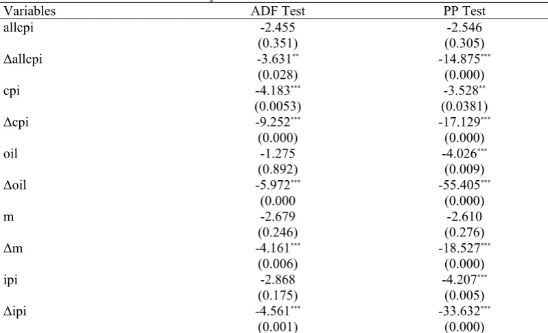
To evaluate the integration properties of the variables, we employ standard augmented Dickey-Fuller (ADF) and Phillips-Perron (PP) tests (Dickey and Fuller, 1981; Phillips and Perron, 1988). A variable is said to be integrated of order d, written I(d) if it requires differencing d times to achieve stationarity. To test for cointegration, we employ the VAR based tests of Johansen (1988) and Johansen and Juselius (1990). Refer Table 3 for the results, which indicates that all variables are I(1).

Table 3: Stationary Tests for CPI and Variable Indicators

Variables ADF Test PP Test

allcpi -2.455 (0.351)

-2.546 (0.305)

Δallcpi -3.631**

(0.028)

-14.875***

(0.000)

cpi -4.183***

(0.0053)

-3.528**

(0.0381)

Δcpi -9.252***

(0.000)

-17.129***

(0.000)

oil -1.275 (0.892)

-4.026***

(0.009)

Δoil -5.972***

(0.000

-55.405***

(0.000)

m -2.679 (0.246)

-2.610 (0.276)

Δm -4.161***

(0.006)

-18.527***

(0.000)

ipi -2.868 (0.175)

-4.207***

(0.005)

Δipi -4.561***

(0.001)

-33.632***

(0.000)

***, **, *

denotes significant at 1 percent, 5 percent and 10 percent respectively. Figures in brackets are p-values. The null for both ADF and PP tests are the hypothesis of a unit root is tested against the alternative of stationarity. The statistics include trend and intercept.

3.2 Illustration of data

1

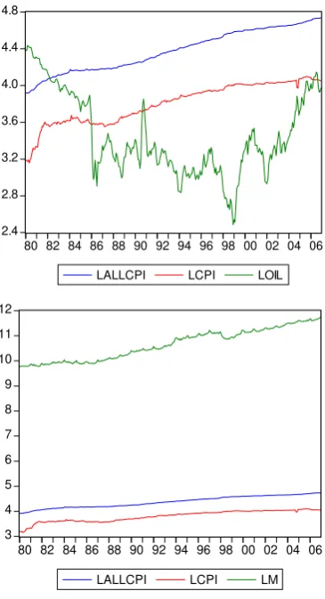
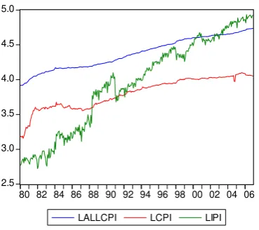
Figure 2 plots CPI and other indicators used to forecast inflation. We use allcpi and cpi as the upper and lower boundary and plot each indicator variable to visually inspect their relationships. The graphs reveal that PPI displays wide gap prior to 1989 and starts to diverge again in 2002. LM indicator shows similar trend2 to CPI and

ALLCPI though the value is higher throughout sample period.

Figure 2: Plots of Indicator Variables within Lower and Upper CPI Bound

2.4 2.8 3.2 3.6 4.0 4.4 4.8

80 82 84 86 88 90 92 94 96 98 00 02 04 06

LALLCPI LCPI LOIL

3 4 5 6 7 8 9 10 11 12

80 82 84 86 88 90 92 94 96 98 00 02 04 06

LALLCPI LCPI LM

2

2.5 3.0 3.5 4.0 4.5 5.0

80 82 84 86 88 90 92 94 96 98 00 02 04 06

LALLCPI LCPI LIPI

4.0 Findings

For the analysis, we divide the findings based on three broad classes of inflation indicators as mentioned earlier.

4.1 Forecasting Results Using Commodity Price

As for Poil, we find that in sub-sample 1-6 there is no cointegration between the indicator and CPI. Only in sub-sample 7 (1980-2004) there exists one cointegrated vector with error correction term, ectt-1, which is negative and significant at one

percent level. This implies that Poil,and CPI are cointegrated in the long run. However, there is no short-run relationship between them since there is nethier uni nor bidirectional causality between the two variables. Refer Table 4 for details. We plot the forecasted CPI using Poil together with actual values of CPI in Figure 3. Overall, since there is only one RMSE result for poil, we report the results. RMSE is 0.0080 and Theil inequality coefficient is 0.70.

Table 4: Results for POIL Indicator Variable Across Sub-samples

Sample Period T, Lag

Cointegration

(Trace test) Granger-causality ectt-1 RMSE

Theil Inequality Coefficient

1. 1980-1992 144, 12 none - - - -

2. 1980 - 1994 174, 6 none - - - -

3. 1980 - 1996 198, 6 none - - - -

4. 1980-1998 222, 6 none - - - -

5. 1980-2000 246, 6 none - - - -

6. 1980-2002 270, 6 none - - - -

7. 1980-2004 295, 5 20.125

[0.009]

- -0.007

[0.0027]

0.0080 0.7043

Note: ectt -1is derived by normalizing the cointegrating vectors on the natural logarithm of the dependent variables, producing

residual r. Figures in (.) and [.] represent t-ratios and p-values, respectively. ***_,**_,* _{denotes significant at 1 percent, 5 percent and}

Figure 3: Plots of forecasted CPI using Poil and actual values of CPI -.04 -.03 -.02 -.01 .00 .01 .02 .03 .04

2005M01 2005M07 2006M01 2006M07

DC PI DCPIF_OIL

DCPIF_OIL+2*SEOIL DCPIF_OIL-2*SEOIL

4.2 Forecasting Results Using Financial Indicator

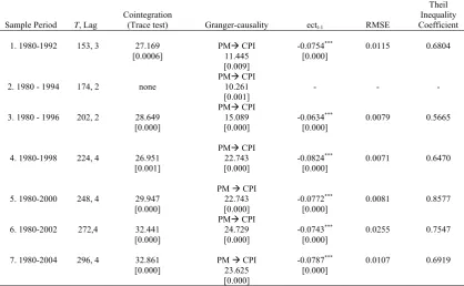
Next, we look at the financial indicators, which are represented by m. We find that six out of seven sub-samples show that there are 6 cointegration between Pm and CPI. In all six cases, we find that the ectt-1 terms are negative and significant indicating the

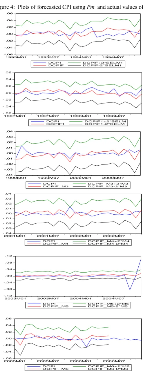
existence of long-run relationship between them. Within these six samples, sub-sample 4 (1980-1988) shows the lowest RMSE of 0.0071 with Theil inequality coefficient equals 0.65. It is also found that in all sub-samples, there exist short run relationship and the causality is running from Pm to CPI at one percent significant level. However, Theil coefficient is quite large which reflects that Pm as forecaster of CPI is not highly accurate. Results are presented in Table 5. The graphical illustration of the actual versus forecasted CPI is displayed in Figure 4.

Table 5: Results for PM Indicator Variable Across Sub-samples

Sample Period T, Lag

Cointegration

(Trace test) Granger-causality ectt-1 RMSE

Theil Inequality Coefficient

1. 1980-1992 153, 3 27.169

[0.0006]

PMÆ CPI

11.445 [0.009]

-0.0754***

[0.000]

0.0115 0.6804

2. 1980 - 1994 174, 2 none

PMÆ CPI

10.261 [0.001]

- - -

3. 1980 - 1996 202, 2 28.649

[0.000]

PMÆ CPI

15.089 [0.000]

-0.0634***

[0.000]

0.0079 0.5665

4. 1980-1998 224, 4 26.951

[0.001]

PMÆ CPI

22.743 [0.000]

-0.0824***

[0.000]

0.0071 0.6470

5. 1980-2000 248, 4 29.947

[0.000]

PM Æ CPI

22.743 [0.000]

-0.0772***

[0.000]

0.0081 0.8577

6. 1980-2002 272,4 32.441

[0.000]

PMÆ CPI

24.729 [0.000]

-0.0743***

[0.000]

0.0255 0.7547

7. 1980-2004 296, 4 32.861

[0.000]

PM Æ CPI

23.625 [0.000]

-0.0787***

[0.000]

0.0107 0.6919

Note: ectt -1is derived by normalizing the cointegrating vectors on the natural logarithm of the dependent variables, producing

residual r. Figures in (.) and [.] represent t-ratios and p-values, respectively. ***_,**_,* _{denotes significant at 1 percent, 5 percent and}

10 percent level, respectively. Cointegration test indicates that there is one cointegrating equation based on Trace statistics. The

Theil inequality coefficient lies between zero and one, where zero indicates a perfect fit. PM Æ CPI indicates PM

Figure 4: Plots of forecasted CPI using Pm and actual values of CPI

-.06 -.04 -.02 .00 .02 .04 .06

1993M01 1993M07 1994M01 1994M07 DCPI

DCPIF

DCPIF+2*SELM1 DCPIF-2*SELM1

-.06 -.04 -.02 .00 .02 .04 .06

1997M01 1997M07 1998M01 1998M07 DCPI

DCPIF1

DCPIF1+2*SELM DCPIF1-2*SELM

-.04 -.03 -.02 -.01 .00 .01 .02 .03 .04

1999M01 1999M07 2000M01 2000M07

DCPI DCPIF_M3

DCPIF_M3+2*M3 DCPIF_M3-2*M3

-.04 -.03 -.02 -.01 .00 .01 .02 .03 .04

2001M01 2001M07 2002M01 2002M07 DCPI

DCPIF_M4

DCPIF_M4+2*M4 DCPIF_M4-2*M4

-.12 -.08 -.04 .00 .04 .08 .12

2003M01 2003M07 2004M01 2004M07 DCPI

DCPIF_M5 DCPIF_M5+2*M5DCPIF_M5-2*M5

-.06 -.04 -.02 .00 .02 .04 .06

2005M01 2005M07 2006M01 2006M07 DCPI

4.3 Forecasting Results Using Real Indicator

All sub-samples, using Pipi as forecaster for CPI traces cointegration vectorsbetween them. Furthermore, the ectt-1 for those sub-samples are negative and highly significant

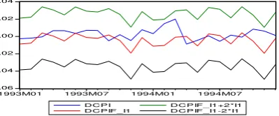
indicating that there is a long run relationship between the indicator and CPI. Granger causality indicates that there is a short run dynamics between them. The sub-sample 4 shows the lowest RMSE of 0.0063. However, Theil coefficient is quite high at 0.61. Refer Table 6 for the details and Figure 5 for the illustrations.

Table 6: Results for PIPI Indicator Variable Across Sub-samples

Sample Period T, Lag

Cointegration

(Trace test) Granger-causality ectt-1 RMSE

Theil Inequality Coefficient

1. 1980-1992 153, 3 15.847

[0.044]

PIPIÆ CPI

9.524 [0.023]

-0.0497***

[0.000]

0.0116 0.7822

2. 1980 - 1994 177, 3 15.931

[0.043]

PIPIÆ CPI

11.717 [0.008]

-0.0439***

[0.000]

0.0068 0.5613

3. 1980 - 1996 201, 3 17.6587

[0.023]

PIPIÆ CPI

12.905 [0.005]

-0.0421***

[0.000]

0.0075 0.5596

4. 1980-1998 224, 4 _17.2295

[0.027]

PIPIÆ CPI

14.446 [0.006]

-0.0514***

[0.000]

0.0063 0.6092

5. 1980-2000 245, 7 21.1389

[0.006]

PIPI Æ CPI 19.991 [0.006]

-0.0.360***

[0.001]

0.0083 0.8752

6. 1980-2002 269, 7 24.1953

[0.002]

PIPI Æ CPI 21.509 [0.003]

-0.0367***

[0.000]

0.0255 0.7999

7. 1980-2004 297, 3 24.5289

[0.001]

PIPIÆ CPI

16.354 [0.001]

-0.0471***

[0.000]

0.0087 0.6834

Note: ectt -1is derived by normalizing the cointegrating vectors on the natural logarithm of the dependent variables, producing

residual r. Figures in (.) and [.] represent t-ratios and p-values, respectively. ***_,**_,* _{denotes significant at 1 percent, 5 percent and}

10 percent level, respectively. Cointegration test indicates that there is one cointegrating equation based on Trace statistics. The

Theil inequality coefficient lies between zero and one, where zero indicates a perfect fit. PIPI Æ CPI indicates PIPI

granger-causes CPI. If the variables are not cointegrated, causality test are conducted with unrestricted VAR.

Figure 5: Plots of forecasted CPI using Pipi and actual values of CPI

-.06 -.04 -.02 .00 .02 .04

1993M01 1993M07 1994M01 1994M07 DCPI

DCPIF_I1

-.05 -.04 -.03 -.02 -.01 .00 .01 .02 .03 .04

1995M01 1995M07 1996M01 1996M07 DCPI DCPIF_I2 DC PIF_I2+2*I2 DC PIF_I2-2*I2 -.05 -.04 -.03 -.02 -.01 .00 .01 .02 .03 .04

1997M01 1997M07 1998M01 1998M07 DCPI

DCPIF_I3

DC P IF_I3+2*I3 DC P IF_I3-2*I3

-.05 -.04 -.03 -.02 -.01 .00 .01 .02 .03 .04

1999M01 1999M07 2000M01 2000M07 D CP I

D CP IF_I4

D C P IF_I4+2*I4 D C P IF_I4-2*I4

-.04 -.03 -.02 -.01 .00 .01 .02 .03 .04

2001M01 2001M07 2002M01 2002M07 DCP I DCPIF_I5 DC PIF_I5+2*I5 DC PIF_I5-2*I5 -.12 -.08 -.04 .00 .04 .08 .12

2003M01 2003M07 2004M01 2004M07 DCPI DCPIF_I6 DCPIF_I6+2*I6 DCPIF_I6-2*I6 -.04 -.03 -.02 -.01 .00 .01 .02 .03 .04 .05

2005M01 2005M07 2006M01 2006M07 D CP I

DCPIF_I7

DCP IF_I7+2*I7 DCP IF_I7-2*I7

Conclusion

Since inflation rate is one of the important indicators of economic well-being and low inflation indicates positive effect on the economy while high inflation gives negative signals to the health of the economy, hence, it is important for the government to predict on the future rate of inflation in order to outline policy measures.

In this paper, we test several inflation indicators in order to identify the best inflation forecaster in Malaysia using the VECM framework. The inflation variables used are the commodity prices, financial indicator and status of the real economy. We find there is no cointegration between commodity price (represented by OIL) and CPI. Although there is some cointegration between financial indicator (represented by M1) and CPI, but we conclude that the best predictor of inflation in Malaysia is industrial production index (IPI) which is the proxy for the economic activities.

References

Bank Negara Malaysia (BNM), BNM Monthly Bulletin, various issues.

Bryan, Michael F. and Cecchetti, Stephen G. 1993. “The Consumer Price Index as A Measure of Inflation,” Federal Reserve Bank of Cleveland Economic Review 29, No. 3.

Cecchetti, Stephen G. et al. 2000. “The Unreliability of Inflation Indicators,” Current

Issues in Economic and Finance, Vol. 6, No. 4. Federal Reserve Bank of New York.

Dickey, D.A. and Fuller, W.A. 1987. “The Likelihood Ratio Statistics for Autoregressive Time series With a Unit Root,” Econometrica, 49(4): pp. 251-76.

Fisher, Jonas D.M. 2000. “Forecasting Inflation With a Lot of Data,” Chicago Fed

Letter, no. 151. March.

Ibrahim, Mansor H. 1996. “Inflationary Behavior in Malaysia: An Empirical Re-Evaluation of its Determinants,” paper presented at 4th Malaysian Econometric Conference, Park Royal Hotel, Kuala Lumpur. 9-10 October, organized by MIER.

Johansen, S. 1988. “Statistical Analysis of Cointegrating Vectors,” Journal of

Economic Dynamics and Control, 12: pp. 231-254.

Johansen, S. and Juselius, K. 1990. “Maximum Likelihood Estimation and Inference on Cointegration with Applications to the Demand for Money,” Oxford Bulletin of

Economics and Statistics, 52(2): pp. 169-210.

Phillips, P.C.B. and Perron, P. 1988. “Testing for a Unit Root in Time Series Regression,” Biometrika, 75(2): pp. 335-346.