An Iteration Method to Solve the Boundary Layer Flow past a Flat Plate

(1)

http://dx.doi.org/10.4236/jamp.2014.24005

How to cite this paper: Kusukawa, K., et al. (2014) An Iteration Method to Solve the Boundary Layer Flow past a Flat Plate.

JournalofAppliedMathematicsandPhysics, 2, 35-40. http://dx.doi.org/10.4236/jamp.2014.24005

An Iteration Method to Solve the Boundary

Layer Flow past a Flat Plate

Ken-ichi Kusukawa1_{, Shigeaki Suwa}2_{, Takeo R. M. Nakagawa}3*

1_{Tokyo Metropolitan University, Hachiohji, Japan} 2_{National Defense Academy, Yokosuka, Japan}

3_{Jusup Balasagyn Kyrgyz National University, Frunze Str. Bishkek, Kyrgyz Republic}

Email:*_{npo.hakusan@kjc.biglobe.ne.jp}

Received 7 January 2014; revised 7 February 2014; accepted 16 February 2014

This work is licensed under the Creative Commons Attribution International License (CC BY). http://creativecommons.org/licenses/by/4.0/

Abstract

An iteration method similar to the thin-wing-expansion method for the compressible flow has been proposed to solve the boundary layer flow past a flat plate. Using such an iteration, the first step of which is Oseen’s approximation, the boundary layer past a flat plate is studied. As pro-ceeding from the first approximation to the second and third approximations, it is realized that our solution approaches to a well known Howarth’s bench mark one gradually. Hence, it is con-cluded that the usefulness of the present method has been confirmed.

Keywords

Boundary Layer Flow; Mathematical Analysis; Iteration Method; Approximate Solution; Navier-Stokes Equation

1. Introduction

For an analytical treatment of the boundary layer flow past a flat plate, one must solve the Navier-Stokes equa-tion under suitable boundary condiequa-tions. But unfortunately, it accompanies a great difficulty to obtain such an analytical solution. Thus, as it is well known, one has proceeded to classify the flow according to whether the Reynolds number is small or large: if the Reynolds number is small, the linearization of Oseen or Stokes type is often employed. Whereas if the Reynolds number is large, the inertia force dominates and so the viscosity is neglected except in the boundary layer [1]-[8]. At high Reynolds number, however, the usefulness of the pro-posed iteration method [9] is not obvious.

(2)

Reynolds number. Even though no exact solution of Navier-Stokes equation for a flat plate at high Reynolds number has been known, boundary layer solution for the flow past a semi-infinite flat plate by Howarth [4] must be a very good approximation to the exact solution. We, therefore, have solved the boundary layer equation, by using the present proposed iteration method.

2. Formulation of Problem

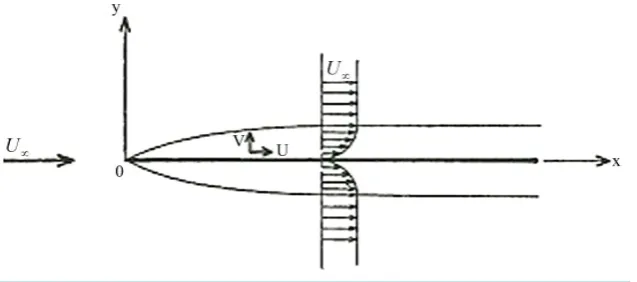
Consider the steady viscous flow past a semi-infinite flat plate at zero incidence placed in the uniform flow ve-locity, U∞. As is shown in Figure 1, we shall take the Cartesian coordinates, x and y, where x-axis is parallel to the flat plate, and the leading edge of the plate is origin of the co-ordinate. The velocity at the potential flow re-gion is assumed to be constant, and thus, dp dx=0, where p is the pressure. It is well known that the boundary layer equations [10] are expressed by

2 2

u u∂ ∂ + ∂ ∂ = ∂x ν u y ν u ∂y , (2.1) 0

u x u y

∂ ∂ + ∂ ∂ = , (2.2) 0, at 0

u= =v y= , (2.3) , at

u=U∞ y= ∞, (2.4)

where u and ν denote the x- and y-components of the velocity, respectively, and ν the kinematic viscosity of fluid.

We shall assume that the velocity components

( )

u,ν may be expanded into the ε-power series such that

2 3

1 2 3

u=U_∞+εu +ε u +ε u +, (2.5)

2 3

1 2 3

ν εν= +ε ν +ε ν +, (2.6) where ε is a small parameter that may be considered as the ratio of the boundary layer thickness to the flat plate length. Substituting (2.5) and (2.6) into (2.1)-(2.4), and rearranging the terms of the same order in ε, we have

2 2

1 1 0

U_∞∂u ∂ − ∂x ν u ∂ =y , (2.7)

(

)

1

2 2 2

1 , for 2

n

n n k k n k k n k

U∞∂u ∂ − ∂x ν u ∂ = −y

∑

=− u ∂u − ∂ + ∂x ν u − ∂y n≥ , (2.8)

0, for 1

n n

u x ν y n

∂ ∂ + ∂ ∂ = ≥ , (2.9)

1 , 1 0, at 0

u = −U∞ ε ν = y= , (2.10)

(

)

0, for 2 at 0

n n

u =ν = n≥ y= , (2.11)

(

)

0, for 1 at

n

[image:2.595.156.475.567.708.2]

u = n≥ y= ∞. (2.12) Equation (2.7) is a modified Oseen’s equation, which is regarded as the first approximation of the boundary layer equation, being obtained by simplifying the Navier-Stokes equation at high Reynolds number.

(3)

3. The First Approximation

Let’s proceed to the first approximation. Introducing the Laplace transform, ū1, of u1 with respect to x, which is defined by

(

)

(

)

1 , ₀ 1 , e d

x

ū λ y =

∫

∞u x y −λ x, (3.1) together with (2.7), we can obtain the equation governing ū1 in the following form

2 2

1 1 0

ū y U ū_∞λ ν

∂ ∂ − = , (3.2) where λ is the parameter of the Laplace transformation. The general solution of (3.2) satisfying (2.10) and (2.12), can be easily be expressed such as

( )

1 exp

U

ū U y

v

λ

ελ ∞

∞

 _ _ 

= − ⋅ _− _ _ _

 

 . (3.3)

By performing the inverse Laplace transformation of ū1, we get

(

)

1 2 1

u =U_∞ ε⋅ Φ_ η − _, (3.4) where Φ

( )

η is the Error function, which is defined as follows,

( )

2

0

2 ηexp t dt

η

Φ = π ⋅

_∫

− , (3.5)

with η= y U_ _∞

( )

νx _1 2. Using (3.4) together with (2.9) and (2.10), we have

( )

1 2

(

₂

)

1 1 U πx 1 exp 4

ν = ε ν⋅ ∞   − −η . (3.6)

These results of (3.4) and (3.6) may be obtainable by the same technique, to be used in the second and the third approximations in Sections 4 and 5.

4. The Second Approximation

The equation of continuity (2.9) for n = 2 can be automatically satisfied by introducing the following stream function,

(

)

1 2

( )

2 xU f2

ψ = ν ∞ η , (4.1)

where f2

( )

η depends on η only. The relevant velocity components are then given, respectively, by

( )

2 2 2

u = ∂ψ ∂ =y U f_∞ ′η ,

(

)

1 2

( )

2 2 x 1 2 U x f2 f2

ν = −∂ψ ∂ = ⋅ν _∞ _η ′ η − η _, (4.2) where f2′

( )

η means the differentiation of f2

( )

η with respect to η.

( )

2 2 2

u x U_∞η x f′′η

∂ ∂ = − ⋅ ,

( )

1 2

( )

2

2 2

u y U_∞ U_∞ νx f′′η

∂ ∂ = _ _ ⋅ ,

( ) ( )

2

2 2

u y U_∞ νx f′′′η

∂ ∂ = ⋅ . (4.3) Substituting (4.2) and (4.3) into (2.8) for n = 2, and using (3.4) and (3.6), we get

( )

2

2 2

2 f′′′η η+ f′′η =G η ε , (4.4) where

( )

(

2

)

{

1 2

(

)

(

2

)

}

exp 4 π 1 2 2π 1 exp 4

(4)

Referring (4.2), the boundary conditions (2.11) and (2.12) for n = 2 can be expressed as follows,

( )

2 2 0, at 0

f η = f′η = η= , (4.6)

( )

2

limη→∞ f′′η =0. (4.7) The solution of (4.4) satisfying the conditions (4.6) and (4.7) is obtainable as

( )

(

)

(

)

(

) (

)

(

)

(

)

( )

(

)

(

)

(

)

(

)

2 2 1 2 2 1 2

2

1 2 1 2 1 2 2 1 2

1 2 2 6 π exp 4 2 1 2 π 2 4 π 2

4 2 π π 4 π 1 1 π exp 4 2 π 4 π 1 π 1 ,

f η ε η η η η η η η

η η η



= ⋅ − Φ_ − ⋅ − Φ + − ⋅Φ − ⋅Φ



+ Φ + − − + + _{− } (4.8)

and

( )

(

)

(

)

(

) (

)

(

) (

)

(

)

2 2 1 2 2

2

1 2 2 1 2 2

1 2 2 π exp 4 2 1 2 π 2

4 π exp 4 π 2 π exp 2 1 .

f η ε η η η η η

η η η



′ = ⋅ −Φ_ + ⋅ − Φ + − Φ



− + − + − _{+ } (4.9)

It may be worth noting here that in the approximation of each order we can introduce the reduced stream function fk

( )

η in such a way,

( )

, with 1, 2,

k k

u =U f_∞ ′η k=  (4.10) On the other hand, the original Equations (2.1) and (2.2) suggest that the velocity component u can be ex-pressed by

( )

u=U f_∞ ′η , (4.11) where f

( )

η is no more than the Blasius’s reduced stream function. Recalling (2.5), we have

( )

2

( )

1 2

f η = +η εf η +ε f η +. (4.12)

5. The Third Approximation

Adopting the similar procedure to Section 4, the equation for f₃

( )

η and the relevant boundary conditions have been reduced to

( )

3

3 3

2f′′′η η+ f′′η =H η ε , (5.1)

( )

3 0, at3 0

f η = f′η = η= , (5.2)

( )

3

limη→∞ f′η =0, (5.3) where

( )

(

)

(

)

(

)

(

) (

)

(

)

(

)

(

)

(

)

(

)

(

) (

)

(

) (

)

(

)

(

)

( )

(

)

2 1 2 2 2 2 2

1 2 3 2 1 2 1 2 2

3 2 2 1 2 2 1 2 2

3 2 2 3 1 2 2 2 2

4 1 π exp 4 2 1π 4 exp 4 2

1π 2 3 2π 2 π 1π exp 4 2

2 π exp 4 2 1π 3 π 4 π 2 exp 2

π exp 3 4 4π 3 2π 2 π 4 π exp 4 ,

H η η η η η η η η

η η η η η η

η η η η η

= + ⋅ − Φ + ⋅ + − Φ

− ⋅ + − + − − Φ

− ⋅ − Φ − ⋅ + − + −

 

+ ⋅ − ⋅ +_ + + − _ −

(5.4)

and

( )

3 3

u =U f_∞ ′η ,

(

)

1 2

( )

3 1 2 U x f3 f3

ν = ⋅ ν _∞ _η ′η − η _. (5.5)

(5)

( )

{

(

)

( )

(

)

(

)

(

)

( )

(

)

(

)

(

)

(

)

(

)

(

)

(

)

(

)

( )

(

)

(

)

(

( )

)

(

)

(

) (

)

( )

(

)

( )

(

)

(

)

( ) (

)

3 3 2 1 2 2 2

3

1 2 2 2 1 2 2

2 1 2 3 2 1 2 2

2 2 3 2

1 2 3 2 1 2

1/ 2 1 2 1 2

1 2 2 8π exp 4 2

27 4π 9 4π exp 4 2 π 1π 2

4π π 6 π 15 2π exp 4 2

2π exp 2 2 2 π 3 4π 3 π 1 2 2

1π 4π 5 2 3 4π 3 2

1 4 2 π 2 2 2 π 5 4 π

f η ε η η η η η

η η η η η

η η η η

η η η η η

η η η

= ⋅Φ + ⋅ − Φ

 

+_ − _ − Φ + − + Φ

 

−_ + − + _ − Φ

+ − Φ + + − + Φ

+ ⋅ − Φ − ⋅ Φ

− ⋅ ⋅Φ Φ + ⋅ − Φ

(

)

( )

(

)

(

)

(

)

(

) (

)

(

)

(

)

( )

(

)

( )

}

1 2

2 1 2 5 2 3 2 3 2 3 2 1 2 2

1 2 2 3 2 2

1 2 2 3 2

1 2 1 2

0 1

2

8π π 4 π 3 2π 6 π 9 4π exp 4

1π 2 2 π exp 2 1 π exp 3 4 2 π 1 1 π 2 π 2 π 3 4π 9 2π 9 8

3 2π 3 π 11 9 2 4π ,

η η η

η η η   +_ + + + − + _ − − ⋅ + − − ⋅ − ⋅   + ⋅ − − ⋅_ + − + _

+ ⋅ − Θ + ⋅ ⋅Θ

(5.6)

with

( )

(

2

)

(

)

0 ₀exp 2 2 d

η

η η η η

Θ =

_∫

− Φ , (5.7)

( )

(

2

) (

1 2

)

1 ₀exp 4 2 d

η

η η η η

Θ =

_∫

− Φ , (5.8) and

( )

{

(

)

(

)

(

)

(

)

(

)

(

)

( )

(

)

(

)

(

)

( )

(

)

(

)

( )

(

)

( )

(

)

(

) (

)

(

)

(

)

3 3 3 1 2 2 1 2 2 2

3

3 1 2 2 1 2 3 2 2

2 2 2 3 2

3 2 1 2 3 2 2 1 2 3 2 2

3 1 2

1 1 2 2 16π exp 4 7 8π exp 4 1π 1 2

8π 2π 5 4π π 1π exp 4 2

4π 3 π exp 2 2 2 π 3 4π 3 π 1 2 2

3 4π 3 2 2 π exp 4 2 4π exp 3 4

16π

f η ε η η η η η η

η η η η η η

η η η η

η η η η η

η

 

′ = ⋅Φ −_ ⋅ − + ⋅ − − + Φ_

 

+_ + + − + _ − Φ

   

−_ + _ − Φ +_ + − + _Φ

− Φ ⋅ + ⋅ − Φ − ⋅ − ⋅

−

( )

(

)

( )

(

)

(

)

}

2 1 2 2 2

2 3 2 2 2

2π 3 8π 4 π 4 π exp 4 4π π 2 π 2 π exp 2 2 π 1 1 π .

η η η

 ₊ ₊ ₋ ₊  ₋     +_ + + − _ − + ⋅ − (5.9)

6. Conclusions

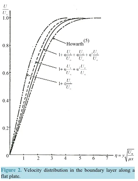
Substituting (3.4), (4.9), (5.9) into (2.5), we obtain the x-component of the velocity. The second and the third approximations for the velocity component have been plotted concurrently in Figure 2. With increasing the de-gree of the approximation, the solution gradually approach to Howarth’s bench mark result. This clearly con-firms the usefulness of the present proposed iteration method to solve the flow past the flat plate.

Introducing dimensionless drag coefficient for the plate wetted on both sides, by the definition [10],

( )

1 2 4 0

f x

C = f′′ R , (6.1) where Rx denotes U x∞ ν , we obtain a formula with (3.4), (4.9), (4.12), and (5.9) as follows,

1 2 1.42

f x

C = R . (6.2) It is found that the Formula (6.2) provides the greater value than that obtained by Blasius’ one [2] slightly, but it is certain that this difference diminishes if we adopt the more higher order approximation.

(6)

U y

x η

µ∞ =

Figure 2. Velocity distribution in the boundary layer along a flat plate.

not always considered to be infinitesimally small, so that much more vigorous mathematical treatment is re-quired to get the solution.

References

[1] Prandtl, L. (1904) Über Flüssigkeitsbewegung bei sehr kleiner Reibung. Verhandl Ⅲ, Intern. Math. Kongr. Heidelberg,

Auch: Gesammelte Abhandlungen, 2, 484-491.

[2] Blasius, H. (1908) Grenzschichten in Flüssigkeiten mit kleiner Reibung. Zeits. f. Math. u. Phys, 56, 1-37.

[3] von Kámán, Th. (1921) Über laminare und turbulente Reibung. ZAMM, 1, 233-252.

http://dx.doi.org/10.1002/zamm.19210010401

[4] Howarth, L. (1938) On the Solution of the Laminar Boundary Layer Equations. Proceedings of the Royal Society of London. Series A, Mathematical and Physical Sciences, 164, 547-579. http://dx.doi.org/10.1098/rspa.1938.0037

[5] Imai, I. (1957) Second Approximation to the Laminar Boundary Layer Flow over a Flat Plate. Journal of the Aero-nautical Sciences, 24, 155-156.

[6] Pohlhausen, K. (1921) Zur näherungsweisen Integration der Differentialgleichung der Grenzschicht. ZAMM, 1, 252- 268. http://dx.doi.org/10.1002/zamm.19210010402

[7] Tani, I. (1954) On the Approximate Solution of the Laminar Boundary Layer Equations. Journal of the Aeronautical Sciences, 21, 487-495. http://dx.doi.org/10.2514/8.3092

[8] Meksyn, D. (1961) New Methods in Laminar Boundary Layer Theory. Pergamon Press, 65-81.

[9] Imai, I. (1944) Two-Dimensional Aero-Foil Theory for Compressible Fluids. Rep. Aero. Research Institute, Tokyo Imperial University, No. 294.

[image:6.595.195.434.78.391.2]