5
VIII
August 2017
Improvement in Execution Time of PSO to Find
Target Object in Running Environment of A*
Algorithm
Pratish Kumar Mahalaha1, Dr. Rajendra Gupta2, Dr. Pratima Gautam3
1Research Scholar, 2Assistant Professor, 3Dean, Dept. of Computer Application AISECT University, Raisen
Abstract: Particle swarm optimization (PSO) is a population based algorithm which is applied to solve many optimization problems. One of the properties of basic PSO is that when particles are spread in a search space, as time increases they tend to converge in a small area. The shortcoming of PSO is that the basic PSO cannot guarantee the global convergence of the algorithm. It means when particles explore different areas, the algorithm do not perform well at exploiting promising areas, which increase the search time. To reduce the search time, A* algorithms is applied to find the target object. This reduces the execution time of PSO. After analyzing the results, it is found that the combination of PSO & A* algorithm give better results. Keywords : Particle Swarm Optimisation, A* Algorithm, path planning
I. INTRODUCTION
The Particle Swarm Optimization (PSO) algorithm is introduced by Kennedy and Eberhart which is one of the self-adaptive global search based optimization technique [8]. The algorithm is very much similar to population-based algorithms like Genetic algorithms. The PSO algorithm relies on the social behavior of the particles in the group. In each epoch, the particle adjusts its trajectory based on its best position which is called local best and the position of the best particle which is called global best of the entire population. This working concept of the algorithm increases the stochastic nature of the particle and congregates quickly global minima with a reasonable better solution.
The popularization of the PSO algorithm is its simplicity and effectiveness in wide range of applications with very low computational cost. Some of the most popular applications that have used in PSO are: the Reactive Voltage Control problem [23], Chemical Engineering [13], Data Mining [16], Pattern Recognition [9] and Environmental Engineering [10]. The PSO algorithm has also been applied to solve NP Hard problems like task allocation [22, 26] and Scheduling [24, 21].
The measurement of similarity in the given problem is used to determine how close two patterns are with one another. The data vectors within a cluster or region have small Euclidean distances from each other and it is associated with one centroid vector, which represents "midpoint" of that clustered area. The centroid vector defined in the algorithm is the mean of the data vectors which belongs to the corresponding cluster area.
In this study, we have analyzed the convergence time of particle swarm optimization (PSO) on the facet of particle interaction. Here we have introduced a statistical interpretation of social only PSO for capturing the essence of particle interaction, which is one of the key mechanisms of PSO. Then we have used the statistical model to find the theoretical results on the basis of convergence time. Since the theoretical analysis of PSO is conducted on the social-only model, instead of on common models in practice, to verify the validity of the results. The numerical experiments are executed on standard functions with a regular PSO program execution.
A. Particle Swarm Optimization Algorithm
searching ability which becomes better when w is smaller. The PSO algorithm with inertia weight factor was called standard PSO. However, in this algorithm, particles would lose the ability to explore new domains when they are searching in solution space. This meaning is to say that it will entrap in local optimization and causes the premature phenomenon. That’s why, it is very import for PSO algorithm to be guaranteed to converge to the global optimal solution and due to this many modified PSO algorithms have been proposed in last ten years.
PSO is a heuristic global optimization method which is developed from swarm intelligence and is based on the research of birds and on the fish flock movement behavior. While searching for food, the birds are either scattered or go together before they find the place where they can get the food. While the birds are searching for food from one place to another, there is always a bird that can smell the food very well. The bird is perceptible of the place where the food can be found, which is having the better food resource information. Since they transmit information, especially the good information at any time, while searching the food from one place to another that’s why it is good for study. The birds will eventually flock to the place where the chances of getting food can be found. As far as particle swam optimization algorithm is concerned, the solution swam is compared to the bird swarm. The birds’ moving from one place to another is equal to the development of the solution swarm, good information is equal to the most optimist solution and the food resource is equal to the most optimist solution during the whole course. The most optimist solution can be worked out in particle swarm optimization algorithm by the cooperation of each individual. The particle without quality and volume serves as each individual, and the simple behavioral pattern is regulated for each of the particle to show the complexity of the whole particle swarm. This algorithm can be used to work out to the complex optimist problems.
PSO algorithm includes many advantages for its simplicity and easy implementations. The algorithm can be implemented widely in the field such as function optimization, machine study, the model classification, neutral network training, vague system control, the signal procession, automatic adaptation control etc.
B. Algorithm for Original PSO
1) Initialize a population array of particles with random positions and velocities on the dimensions D (variable) in the search space.
2) starting the loop
3) For each particle, evaluate the desired optimization fitness function in D.
4) Compare particle’s fitness evaluation with pbesti . If the current value is better than pbesti, then set the pbesti equal to its current value, and pi equal to the current location xi in D-dimensional space.
5) Identify the particle in the neighborhood with the best success so far, and assign its index to the variable g. 6) Change the position of the particle and its velocity according to the following equation :
7) If a criterion is met (sufficiently good fitness or a maximum number of iterations), then exit loop.
8) Loop ending
The meaning of nomenclatures is as given below:
– The function U(0, φi ) represents a vector of random numbers which is uniformly distributed in [0, φi ] that is randomly
generated at each iteration and for each particle. – is component wise multiplication
– Each component of vi is kept within the range [−Vmax to +Vmax]
The basic PSO algorithm described above uses a small number of parameters that are needed to be fixed. One parameter is based on the size of the population. This is often set empirically on the basis of the dimensionality and perceived difficulty of a problem. The values taken in the algorithm, in the range 30–50, are quite common.
In standard PSO, each particle is selected for updating in turn. A complete iteration in the process corresponds to a single position update of each particle. Moreover, in a general swarm model, particles could be chosen at random or according to a selection scheme which is perhaps similar to parent selection in evolutionary computation.
More and more research is needed to clarify the issues of PSO in both type of PSO like classical velocity-dependent and bare-bone type of PSOs. A distinction is made between the memory of the best particle in the neighborhood and the particle’s own memory. It is investigated that the much exploration of particle dynamics is found with many PSO variants borrowing from the wide range of particle interactions in physical systems. For example, the study has been explored the use of spherical particles, sliding (rather than flying) particles, inter-particle repulsive forces and quantum effects. However, so many other types of physical interactions remained unexplored. Moreover, whilst it does looks like that the inclusion of randomness in the form of random force parameters, or sampling from a distribution, is very much useful, which is not known if stochasticity is strictly necessary for good performance. So far, a completely deterministic algorithm has eluded by researcher.
Finally, we can say that occasionally the particles may move to regions at very large distances from the main swarm or even outside the search space.
C. A* Algorithm Algorithm
A* is also pronounced as AStar, is one of the type of search algorithms. A number of problems can be solved by representing the system in its initial state and then for each action it can be performed on the system. The A* algorithm added the features of uniform-cost search and pure heuristic search to proficiently compute optimal solutions. A* algorithm is also called a best-first search algorithm in which the cost is associated with a node. It is represented by the following formula
f(n) = g(n) + h(n)
where g(n) is the cost of the path from the initial state to node n and h(n) is the heuristic estimate or the cost or a path from node n to a goal.
Therefore f(n) estimates the lowest total cost of any solution path going through node n. At each point, a node with lowest f value is chosen for expansion. The ties among nodes of equal value of f should be broken in the favor of nodes with lower h values. The algorithm can be terminated when a goal is chosen for expansion.
The A* algorithm guide an optimal path to a target if its heuristic function h(n) is admissible. The meaning of the statement is that it never overestimates actual cost. It can be explained with an example of airline. Since airline distance never overestimates actual highway distance, and manhatten distance never overestimates actual moves in the gliding tile.
For an Puzzle, the A* algorithm uses evaluation functions, can be find optimal solutions to the problems. Moreover, A* makes the most efficient use of the given heuristic function in the following way;
Among all the shortest-path algorithms uses the given heuristic function h(n). The A* algorithm expand the fewer number of nodes. The problem with A* algorithm is memory requirement. Since the entire open list must be saved at somewhere, A* algorithm is found to be space-limited in practice. It is no more practical than best-first search algorithm on current machines.
D. Limitations of the Existing System
The PSO and A* algorithm are having its own advantags and disadvantages but it tends to be trapped in a local optimum under some initialization conditions. It is noticed that when the maximum number of iterations has been exceeded from its limit, there is little change in the centroid vectors over a number of iterations and even when there are no cluster membership changes. In the proposed method, the algorithm is stopped when a user-specified number of iterations have been exceeded. The earlier method are having following limitations :
1) The proposed method easily suffers from the partial optimism that causes less exact at the regulation of its speed and the direction.
2) The method can’t work out the problems of scattering and optimization 3) The method can’t work out the problems of non-coordinate system.
II. OBJECTIVE
A. To improve the execution time of PSO
B. To reduce the total path finding time in PSO-AStar
III. LITERATURE REVIEW
PSO algorithm has an acceptable and given better performance in the searching task. In several instances of adaptations of PSO have been used for multi-robot odour searches [9, 10].
The successful and adapted version of PSO on distributed mobile robots has been used to search the environment based on local information only [2, 11]. The successful implemented versions of PSO show that their performance in a group of robots is much better than the basic PSO algorithm. However, it is seen that the adapted version has its shortcomings and limitations, particularly when placed in an environment with a higher number of obstacles. One of the main problem of PSO is its premature convergence. It means that the particles have a tendency to move towards the best location found and converge to that area. Therefore, it has exploitative behaviour over time spam. It is noticeable that the global searching of PSO decreases as the time progresses.
The problem of premature convergence of PSO algorithm is also an evident in the multi robot search system in its environments that contain static obstacles. In other words, we can say that one of the basic PSO properties is that the global searching or exploration of machine decreases over time and they converge to a small area and then it becomes unable to explore other promising areas. This problem is called premature convergence. In this situation, when there are big obstacles in an environment found then these static obstacles amplify the problem. These obstacles are bigger and taller than the robotic machine and so prevent it from observing the environment behind them. When the target is placed near the obstacles, the probability of observing from the other side of the obstacles becomes low, and as time increases, the global searching of the robots decreases gradually. As a result the algorithm searches the small area continuously and converges to that small area without being able to search the other promising areas. On the basis of PSO algorithm, the robots’ velocities in the early iterations are high due to their greater inertia weight. Therefore, the global searching and exploration of the robots becomes higher than that of local searching and exploitation. With the increase in time, the inertia weight value decreases slightly which leads to a decrease in the global searching of PSO algorithm. However, the robots may converge to the area that may not be contained the given target. Some studies has been done run on multi-robot search systems to solve this premature convergence problem.
In [16] two new methods have been proposed which are based on Particle Swarm Optimization (PSO) and Darwinian Particle Swarm Optimization (DPSO) respectively. These two emerging methods are adapted to multi-robot search systems where obstacle avoidance is of high priority. The outcomes of the study determined that RDPSO increases the search exploration to avoid being stuck in local optima and a rapid convergence to the desired objective value in comparison to RPSO. In the study it is found that the problem of basic PSO is the lack of guarantee in global convergence. While establishing an efficient balance between exploration and exploitation is the drawback of basic PSO algorithm. The earlier studies have been proposed several methods to solve type of problem in different domains [17, 18].
In [19], one more method is proposed MPSO, which is based on Multi-robot Search System. In this method, they added the local search method to the PSO and established a balance between exploration and exploitation. According to this, the robots are deployed in the search space and look for the target. When the robot check the target, the value of fitness function is calculated in parallel, and if the value of fitness function in its current position exceeds half of the goal fitness function value, the robot uses the local search strategy instead of basic PSO. In addition to this the environment does not contain any big obstacles that prevent the robots from observing the area surrounding the static obstacles. Therefore, there are no areas found where the robot becomes stuck and after a while converges to that area.
In the further study, a simple and effective PSO algorithm has been proposed that is ‘Modified PSO with Local Search (ML-PSO)’. ML-PSO is based on the modification of basic PSO developed by [20]. The algorithm is applied in the exploration search space. A new method is proposed in this study for multi-robot search system which increases the global searching and guides the robot to escape from the local optima and explore different areas to find the desired target. This attempt is made to solve two problems; premature convergence through increasing the global searching of robotic machine and adding a local search algorithm such as A-star to guarantee global convergence with a reduction in the search time.
Deelman et al. [5] have done study on planning, mapping and data-reuse in the area of workflow scheduling. The author has proposed Pegasus [5], which is one of the framework that maps complex scientific workflows onto distributed resources such as the Grid. The Taverna study [12] has developed a system tool for the composition and enactment of bioinformatics workflows for the life science community. One other well-known study on workflow systems includes GridFlow [4], GridAnt [1], ICENI [6], Kepler [11] and Triana [18]. The author terms this as “Best Resource Selection (BRS)” approach, where a resource is selected based on its performance.
IV. PROPOSED METHODOLOGY
data mining algorithms, where prior to, and during training period, training data is clustered or partitioning of the area. Samples from clusters are selected as training data, thereby reducing the computational complexity of the training process so as to improving generalization performance. The algorithm is then extended to use clustering or partitioning to seed the initial swarm. This extended algorithm basically uses PSO to refine the clusters.
The clustering algorithm tends to converge faster as compared to PSO, but generally with less accurate clustering. This study shows that the performance of the PSO clustering algorithm can be further improved by seeding the initial swarm with the result of the K-means algorithm.
The hybrid algorithm first executes the K-means algorithm once. The aim of the PSO is to find the particle position that results in the best evaluation of a given fitness objective function.The Proposed algorithm is an advancement of A* algorithm using PSO. According to this algorithm, the algorithm is modified in two aspects.
A. No. of List Used
A* algorithm uses two lists namely Open and Closed list (open list is for all exploring nodes and closed list is for all selected nodes) Our approach uses only closed list which mean only selected co-ordinates are stored for drawing the path.
B. No. of Path Found
1) In A* algorithm, only path is found during the execution of iterations.
2) The proposed method found many paths depending on the number of valid adjacent nodes (particles) of the start node. 3) If there are n valid adjacent nodes of start node then it finds n number of path.
The optimal path is selected based on the total distance covered by all the paths. Object reaches the target in less time. The pseudo code of enhanced PSO algorithm using A* algorithm is summarized as follows:
Step 1: Initialize the size of the population N
Initialize the dimension of the solution space D Initialize the maximum number of iterations K Initialize the inertia weight start w and end w Initialize the obstacles O
Initialize OpenList and CloseList Step 2: N = N - Obstacles
Step 3: for each particle
Initialize the particle position Xi randomly
Initialize the particle velocity Vi randomly
Initialize the current position as Pi
Evaluate the fitness value
Initialize Pg according to the fitness value
Step 4: Calculate new inertia weight Step 5: Update velocity of each particle, If (Vid> Vmax’) then Vid = Vmax If (Vid< -Vmax’) then Vid = -Vmax Step 6: Update position of each particle, If (Xid> Xmax’) then Xid = Xmax If (Xid< Xmin’) then Xid = Xmin
Step-7: Explore all nodes from start node to target node and store in OpenList
Step 8: Evaluate the fitness values of all particles. For each particle, compare its current position If (Pi fitness > pbest) then pbest=Pi; Update Fitness Value
If (Fitness value of Pi> Fitness of gbest) then
update gbest and its fitness value with the position and objective value of the current best particle.
If (Cost Evaluation Function f(n) Value is Less) Then Select this node and store in ClosedList
a) Working principle of PSO – A* algorithm
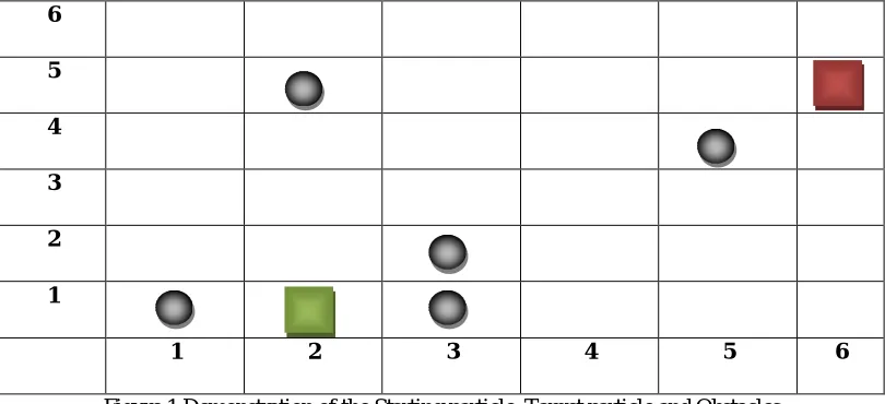
Step 1: Initialize the map with starting and target point, obstacles position etc. (in the following figure, green box shows the starting
position, red box is target and grey circles denote obstacles.
6
5
4
3
2
1
[image:7.612.104.509.115.300.2]1 2 3 4 5 6
Figure 1Demonstration of the Starting particle, Target particle and Obstacles
Step 2:Place the particles in every valid node (not include the obstacles and target) which touches the boundary of start node, these nodes becomes particle node.
6
5
4
3
2 P2 P1
1
[image:7.612.104.510.334.518.2]1 2 3 4 5 6
Figure 2 Location of the particles and path searching Step 3:For each particle node
3.1) Find all nearby valid possible nodes of this particle node and name it as current node.
6
5
4
3 C3 C2 C1
2 P2 P1
1
Figure 3Analysis of nearby clusters and finding the low cast of the particle 3.2) Apply the cost evaluation function and find the distance.
3.3) Function is applied between particle’s node and goal node.
• Calculate f(n) for C1 and C2 and choose the minimum cost node. F(n) = g(n) + h(n) • Co-ordinates of P1 (2,2) , C1(3,3), C2(2,3) and T(6,5).
• F(n) for C1 is
• g(1) = 1.41, h(1) = 3.60, then f(1) =5.01 • F(n) for C2 is
• g(2) = 1, h(2) = 4.47, then f(2) = 5.47
• The calculated cost comes from node C1 is minimum, so this node is selected and respective co-ordinates are stored in 2-D array and cost value is stored in 1-D array.
3.4) Choose the minimum distance and make that current node as first node.
6
5
4
3 C3 C2 C1
2 P2 P1
1
1 2 3 4 5 6
Figure 4 Particle P1 denoting low cast cluster C1
3.5) Store the co-ordinates of first node in closed list and distance in 1-D array. 3.6) Make this first node as particle node.
6
5
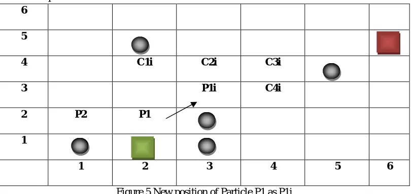
4 C1i C2i C3i
3 P1i C4i
2 P2 P1
1
[image:8.612.105.510.504.696.2]1 2 3 4 5 6
Figure 5New position of Particle P1 as P1i 3.7) Repeat step from 3.1 to 3.5 until particle node is not equal to target node.
6
5 P1k
4 P1j
3 P1i
2 P2 P1
1
[image:9.612.103.508.73.254.2]1 2 3 4 5 6
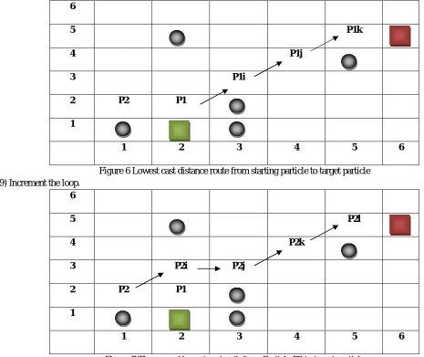
Figure 6 Lowest cast distance route from starting particle to target particle 3.9) Increment the loop.
6
5 P2l
4 P2k
3 P2i P2j
2 P2 P1
1
[image:9.612.49.514.75.466.2]1 2 3 4 5 6
Figure 7The second lowest cast path from Particle P2 to target particle Step 4: Examine the Sum array and find the minimum value,
Step 5: Fetch the co-ordinates from 2-D array with respect to the value comes from step 4 Step 6: Path from start node to target node is drawn with the co-ordinates comes from step 5. Step 7: Show the resultant map, and display the total distance and execution time.
Step 8: Stop the algorithm.
6
5
4
3
2
1
[image:9.612.99.511.541.722.2]1 2 3 4 5 6
V. RESULT AND DISCUSSION
The PSO-AStar algorithms are written in Visual Studio 2010. All experiments are run on Intel-R Duel Core 2.4 GHz Pentium PC machine with 4 GB RAM under Windows-XP Operating System.
Table-1: Execution time of PSO Algorithm with different particles
Particles PSO Execution Time (ns)
10 156285
20 426336
30 656251
40 781288
50 937567
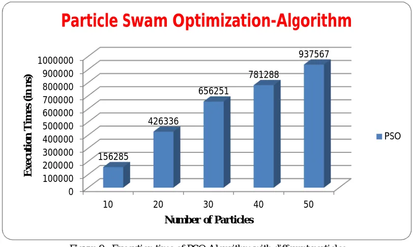
[image:10.612.208.405.128.221.2]The Table 1 shows the execution time of PSO algorithm with different particles. The execution time of 10 particles is 156285 ns, 20 particles is 426336 ns, 30 particles is 656251 ns, 40 particles is 781288 ns, and 50 particles is 937567 ns.
Figure 9 : Execution time of PSO Algorithm with different particles Here execution time is frequently increases when the particles are also increases.
Table-2: Execution time of PSO-AStar Algorithm with different particles and obstacles
Particles PSO-Astar
10 156243
20 156285
30 341772
40 468771
50 781288
The Table 2 shows the execution time of PSO-AStar algorithm with different particles and five obstacles. The execution time of 10 particles is 156243 ns, 20 particles is 156285 ns, 30 particles is 341772 ns, 40 particles is 468771 ns, and 50 particles is 781288 ns.
0 100000 200000 300000 400000 500000 600000 700000 800000 900000 1000000
10 20 30 40 50
156285
426336
656251
781288
937567
Ex
e
c
u
ti
o
n
Ti
m
e
s
(i
n
n
s)
Number of Particles
Particle Swam Optimization-Algorithm
[image:10.612.102.508.273.516.2]Figure 10 : Execution time of PSO-AStar Algorithm with different particles and obstacles
The Figure 10 shows the execution time of PSO-AStar algorithm with different particles and five obstacles. The execution time of 10 particles is 156243 ns, 20 particles is 156285 ns, 30 particles is 341772 ns, 40 particles is 468771 ns, and 50 particles is 781288 ns. Here execution time is frequently increases when the particles are also increases. Here the execution time is less as compare to classic PSO Algorithm. If obstacles are increases then execution time is also reduce.
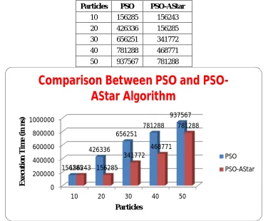
Table-3: Comparison of Execution time between PSO and PSO-AStar Algorithm with different no. of particles
Particles PSO PSO-AStar
10 156285 156243
20 426336 156285
30 656251 341772
40 781288 468771
50 937567 781288
Figure 11: Comparison of Execution time between PSO and PSO-AStar Algorithm with different no. of particles
0 100000 200000 300000 400000 500000 600000 700000 800000
10 20 30 40 50
156243 156285 341772 468771 781288 Ex e c u ti o n Ti m e (i n n s)
Number of Particles
PSO-AStar Algorithm
PSO-AStar 0 200000 400000 600000 800000 100000010 20 30 40 50
156285 426336 656251 781288 937567 156243 156285 341772 468771 781288 Ex e c u ti o n Ti m e (i n n s) Particles
Comparison Between PSO and
PSO-AStar Algorithm
PSO
[image:11.612.118.501.408.718.2]The Figure 11 shows the execution time between PSO algorithm and PSO-AStar algorithm with different no. of particles. Here PSO-AStar always takes less execution time as comparison with basic PSO algorithm in nano seconds (ns).
The proposed algorithm minimizes the following limitations of PSO algorithm: A. This approach does not use the concept of open list.
B. Open list require more maintenance time because it stores the co-ordinates of unselected nodes and they are approx 6 to 8 times more than selected nodes.
C. In PSO, the position and velocity of particle is updated by an equation, and this is updated in each and every step, so it consume more time.
So, by combining both this algorithm PSO and A*, we find the shortest path in very less time.
VI. CONCLUSION
This paper present a strategy of object movement path planning in dynamic environment with fixed position of obstacles and target points in order to reduce the total path finding time. The comparative results shows that the durability and fastness of the proposed method over the traditional A* algorithm shows better result.
During the result analysis, we have presented our performance study over various objects (i.e. 10, 20, 30, 40 and 50 objects). We also analysed the experimental results of both PSO with AStar (proposed name PSO-AStar) in comparison to an existing PSO algorithm with different particles size.
In the next step of the work, we have planned a strategy of object path planning in dynamic environment with fixed position of obstacles and target points in order to reduce the total path finding time.
The comparative results shows that the durability and fastness of our proposed method over the basic PSO algorithm. The motivation of the study was based on providing solution to the path planning problem with actual applications.
The proposed algorithm PSO-AStar always perform better in terms of execution time as comparison to classic PSO algorithm in nano seconds (ns). The algorithm also produces the best local optima means personal best (pBest) for finding the shortest path planning.
REFERENCES
[1] Chen Yonggang, Yang Fengjie, Sun Jigui (2015) “A new Particle swam optimization Algorithm”, Journal of Jilin University, 2006, 24(2):181-183.
[2] Clerc M, Kennedy J. (2015) “The particle swarm-explosion stability, and convergence in a multidimensional complex space”, IEEE Transactions on
Evolutionary Computation 6(1) : 58-73
[3] Clerc M. (2014) “The swarm and the queen : towards a deterministic and adaptive particle swarm optimization” Proceedings of the Congress on Evolutionary
Computation. Piscataway, NJ : IEEE Service Center : 1951-1957.
[4] Colorni A, Dorigo M, Maniezzo V (2012) “Distributed optimization by ant colonies” Proceedings of the 1st European Conference on Artificial
Life,1991:134-142
[5] Dorigo M, Maniezzo V, Colorni A. (2008) “Ant system : optimization by a colony of cooperation agents” IEEE Transactions on Systems. Man and
Cybernetics-Part B,1996, 26(1):29-41.
[6] Duan Haibin (2007) “Ant Colony Optimization theory and Application” Science Publishing Company of Beijing, 2007.
[7] Eberhart R C, Shi Y. (2007) “Comparison between genetic algorithms and Particle Swarm Optimization” Porto V
[8] W, Saravanan N, Waagen D “Evolutionary Programming VII” [S.l.]: Springer, 2012:611-616
[9] Eberhart R C, Shi Y. (2012) “Comparing inertia weights and constriction factors in Particle Swarm Optimization” Proceedings of the Congress on Evolutionary
Computating, 2006: 84-88.
[10] Eberhart R, Kennedy J. (2002) “A New Optimizer Using Particle Swarm Theory” Proceedings of 6th International Symposium on Micro Machine and Human
Science, Nagoya, Japan. IEEE Service Center Piscataway NJ, 2002 : 39-43.
[11] Gao Ying, Xie Shengli (2004) “Particle swam optimization Algorithm based on Simulated Annealing Approach”, Computer Engineering and Application,
40(1):47-49.
[12] Higashi N, Iba H. (2003) “Particle Swarm Optimization with Gaussian mutation” Proceedings of the 2003 Congress on Evolutionary Computation. Piscataway,
NJ : IEEE Press, 2003:72-79.
[13] Kennedy J, Eberhart R. (2001) “Particle Swarm Optimization”, Proceedings of IEEE International Conference on Neural Network, Perth, Australia, IEEE
Service Center Piscataway NJ, 2001:1942-1948.
[14] Agrafiotis, D. K., & Cedeño, W. (2001) “Feature selection for structure-activity correlation using binary particle swarms”, Journal of Medicinal Chemistry,
45(5), 1098–1107
[15] Angeline, P. (2000) “Evolutionary optimization versus particle swarm optimization: Philosophy and performance differences”, In V. W. Porto, N. Saravanan,
D. Waagen, & A. E. Eiben (Eds.), Proceedings of evolutionary programming VII, pp. 601–610. Berlin: Springer.
[17] Blackwell, T. M. (2003a) “Particle swarms and population diversity I: Analysis”, In A. M. Barry (Ed.), Proceedings of the bird of a feather workshops of the genetic and evolutionary computation conference (GECCO), pp. 103–107, Chicago. San Francisco: Kaufmann
[18] Blackwell, T. M. (2003b) “Particle swarms and population diversity II: Experiments”, In A. M. Barry (Ed.), Proceedings of the bird of a feather workshops of
the genetic and evolutionary computation conference (GECCO), pp. 108–112, Chicago. San Francisco: Kaufmann.
[19] Blackwell, T. M. (2005) “Particle swarms and population diversity” Soft Computing, 9, 793–802.
[20] Doctor, S., Venayagamoorthy, G. K., & Gudise, V. G. “Optimal PSO for collective robotic search applications”, Paper presented at Congress on Evolutionary
Computation, CEC 2004.
[21] Pugh, J., Segapelli, L., & Martinoli, A. “Applying aspects of multi-robot search to particle swarm optimization. International Workshop on Ant Colony
Optimization and Swarm Intelligence”, Brussels, Belgium, 2006, pp. 506-507.
[22] Das, A., Kantor, G., Kumar, V., Pereira, G., Peterson, R., Rus, D., Singh, S., & Spletzer, J. “Distributed search and rescue with robot and sensor teams” Field
and Service Robotics, 2003, Japan.
[23] Di Chio, C., Poli, R., & Di Chio, P. “Extending the particle swarm algorithm to model animal foraging behavior”, International Workshop on Ant Colony
Optimization and Swarm Intelligence, Brussels, Belgium, 2006, pp. 514-515
[24] Sahin, E. “Swarm robotics: From sources of inspiration to domains of application”, In Swarm Robotics: State of-the-Art Survey Ser. Lecture Notes in
Computer Science (LNCS 3342), E. Sahin & W. Spears, Eds. Berlin Heidelberg: Springer-Verlag, 2005, pp. 10–20.
[25] Eberhart, R., & Kennedy, J. “A new optimizer using particle swarm theory” Proceedings of the Sixth International Symposium on Micro Machine and Human
Science, 1995, MHS'95.
[26] Kennedy, J., & Eberhart, R. “Particle swarm optimization:, Proceedings of IEEE International Conference on Neural Networks, 1995.
[27] Hereford, J. M. “A distributed particle swarm optimization algorithm for swarm robotic applications”, Study presented at the IEEE Congress on Evolutionary
Computation, CEC 2006.
[28] Jatmiko, W., Sekiyama, K., & Fukuda, T. “A PSO based mobile sensor network for odor source localization in dynamic environment: Theory, simulation and
measurement”, IEEE Congress on Evolutionary Computation, 2006, CEC.
[29] Marques, L., Nunes, U., & de Almeida, A.T. “Particle swarm-based olfactory Guided Search”, Autonomous Robots, 2006, 20(3), 277-287.
[30] Pugh, J., & Martinoli, A. “Inspiring and modeling multi-robot search with particle swarm optimization”, IEEE Swarm Intelligence Symposium, 2007, SIS
2007.
[31] Shi, Y., & Eberhart, R.C. “Fuzzy adaptive particle swarm optimization” Proceedings of the 2001 Congress on Evolutionary Computation, 2001.
[32] Lovbjerg, M., Rasmussen, T.K., & Krink, T. “Hybrid particle swarm optimiser with breeding and subpopulations” Proceedings of the Genetic and Evolutionary
Computation Conference, 2001.
[33] Ciuprina, G., Ioan, D., & Munteanu, I. “Use of intelligent-particle swarm optimization in electromagnetic” IEEE Transactions on Magnetics, 2002, 38(2),
1037-1040.
[34] Clerc, M. “The swarm and the queen: Towards a deterministic and adaptive particle swarm optimization” Proceedings of the 1999 Congress on Evolutionary
Computation, 1999, CEC 99.
[35] Couceiro, M.S., Rocha, R.P., & Ferreira, N.M. “A novel multi-robot exploration approach based on particle swarm optimization algorithms”, IEEE
International Symposium on Safety, Security, and Rescue Robotics (SSRR), 2011.
[36] E. Deelman, G. Singh, M.-H. Su, J. Blythe, Y. Gil, C. Kesselman, G. Mehta, K. Vahi, G. B. Berriman, J. Good, A. Laity, J. C. Jacob, and D. S. Katz. Pegasus
“A framework for mapping complex scientific workflows onto distributed systems”, Sci. Program., 13(3):219–237, 2005.
[37] N. Furmento, W. Lee, A. Mayer, S. Newhouse and J. Darlington. “ICENI: an open grid service architecture implemented with JINI In Supercomputing’02”
Proceedings of the 2002 ACM/IEEE conference on Supercomputing, 2002.
[38] Y. Gil, E. Deelman, M. Ellisman, T. Fahringer, G. Fox, D. Gannon, C. Goble, M. Livny, L. Moreau, and J. Myers “Examining the challenges of scientific
workflows” Computer, 40(12), 2007.
[39] J. Kennedy and R. Eberhart “Particle swarm optimization” In IEEE International Conference on Neural Networks, volume 4, pages 1942–1948, 1995.
[40] J. Louchet, M. Guyon, M. J. Lesot, and A. Boumaza “Dynamic flies: a new pattern recognition tool applied to stereo sequence processing”, Pattern Recognition
Letters, 23(1- 3) : 335–345, 2002.
[41] W. Z. Lu, H. Y. Fan, A. Y. T. Leung, and J. C. K. Wong “Analysis of pollutant levels in central Hong Kong applying neural network method with particle
swarm optimization”, Environmental Monitoring and Assessment, 79(3):217–230, Nov 2002.
[42] B. Ludascher, I. Altintas, C. Berkley, D. Higgins, E. Jaeger, M. Jones, E. A. Lee, J. Tao, and Y. Zhao “Scientific work-flow management and the kepler