Effects of Sensor Nodes Mobility on Routing Energy
Consumption Level and Performance of Wireless Sensor
Networks
Mina Malekzadeh
Golestan University
Zohre Fereidooni
Golestan University
M.H. Shahrokh Abadi
Electrical and Computer Faculty Hakim Sabzevari
University
ABSTRACT
Due to wireless sensor networks (WSN) characteristics, routing in these networks is a challenging task particularly when the wireless nodes, which are energy constrained, are moving. Mobility in WSNs can cause frequent route changes or breaks. In case of route breaks, each routing protocol reacts differently which in turn cause a different pattern in the energy consumption. Therefore, it is important to consider the impact of mobility on energy level of sensor nodes to select a proper routing scheme for a particular WSN. In this paper, an attempt has been made to measure energy consumption level of the sensor nodes while moving through the WSN environment on different locations. The main contribution of this paper is to compare and analyze performance of the mobile nodes using two well-know routing protocols, DSR and AODV, in terms of three performance metrics as energy efficiency, packet delay, and packet lost rate. The comparison has been done using NS2 network simulator.
Keywords
Sensor mobility, energy efficiency, energy consumption level
1.
INTRODUCTION
Nowadays wireless sensor networks (WSN) are widely deployed to monitor and examine different phenomena in variety areas including nature, home automation, industrial and military applications. To achieve their goals, WNSs are composed of several wireless nodes communicating to each other. The wireless sensor nodes are mainly powered by small batteries as their source of energy, which has limited the lifetime of WSNs. Due to WSN characteristics, there are different factors affecting lifetime of WSNs. Among them, three factors as type of routing protocols, sensor nodes mobility, and topology states are the main focus of this paper.
a. Type of routing protocols: type of routing protocol affects the energy consumption due to different routing process and overhead. Routing is a process to establish and maintain routes and move packets between source and destination more quickly and efficiently. Two common routing algorithms used in WSNs are Ad Hoc On-demand Distance Vector (AODV) and Dynamic Source Routing (DSR).
AODV protocol: When a source node S needs a route to destination node D, it broadcasts a ROUTE REQUEST message to all its neighbors. The message includes information such as source IP, destination IP, lifespan of the message, and destination Sequence Number (SN). The SN helps in identifying the freshness of the route to the
greater than or equal to it, then that node generates a ROUTE REPLY that contains the number of hops for D. Since there might several nodes send back the ROUTE REPLY, the needy node s uses the route that has the least number of hops to the destination and greater sequence number, over the other nodes. Thus, AODV determines the rout from source to destination by independent hop-by-hop routing decisions made by each node. Any intermediate node always tries to keep a list of all its next hops.
DSR protocol: a complete ordered list of nodes information for the path from the source to the destination is included in the header of the request. A given intermediate node simply forwards data packets to the specified next node. The sender identifies the entire route node into which the packet has to pass through to reach the destination. Then the sender lists the route in the packet’s header so that the next intermediate node can be identified by the address on the way to the destination host. Fresh routing information is not needed to be maintained in intermediate nodes since all the routing decisions are contained in the packet by themselves. This results in less routing overhead for DSR than AODV.
b. Sensor nodes mobility: a mobile node in WSN is a sensor whose location may frequently be changed. Mobility effects can vary widely including changing network density and stability, service availability of the sensor nodes, number of average connected routes which in turn affects the number of hops and performance of the routing algorithms.
c. Topology states: the state of topology can be either dynamic or static which is directly related to existence of either mobile or stationary sensor nodes in the network respectively.
The rest of the paper is organized as follows. Section 2 surveys related works. In Section 3 the proposed simulation scheme and scenarios are presented. Section 4 presents and discusses our simulation results. Section 5 concludes the work.
2.
RELATED WORKS
Pandey et al. [1] compared AODV and DSDV through an analytical model. The results prove the correlation between routing energy consumption with topology change rates and traffic conditions. However, their work differs from ours in different aspects such as implementation and modeling of the energy consumption, simulation tool, and the performance metrics.
In [2], authors analyzed the performance of several routing protocols on the basis of throughput, average delay, and routing overhead. To provide comparison, different scenarios are performed including variation of number of nodes, pause time and mobility. However the energy consumption level in these variations is not considered.
In [3], the focus is on three types of routing protocols AODV, HYBRID, and DSDV. The comparison is done based on packet delivery ratio and average end to end delay in java environment. Aside from the simulation environment, it differs from ours in both the routing protocols and mobility model.
Kulkarni et al. [4] compared the performance of three routing techniques AODV, DSDV, and DSR in different way. The major parameters for their performance study are based on the node deployment, total energy consumption, and the coverage area.
In [5], the goal was to investigate the relationship between the mobility and energy consumption of the routing protocols, whereas the authors concentrated on the impact of the traffic conditions, speed, and node numbers.
Most of the previous works [6-10] focus on performing simulations in terms of packet delivery fraction, average delay, and number of dropped data packets while mobility and energy consumption level are not investigated.
3.
SIMULATION MODEL
In this section, we describe the implementation details of our WSN topology, scenario models, and the performance metrics to evaluate the models.
3.1.
Network model
The simulations in this research are performed using NS2. XGraph utility is used to plot the graphs in NS2. We consider WSN in a surface of 1000m x 1000m at which the nodes are randomly distributed. A mobility model in WSN shows the movement pattern of the sensor nodes in the network. The basic energy model is determined by the class EnergyModel in NS2. We have chosen Random Waypoint (RWP) as the mobility model through this work which is commonly used in most simulations.
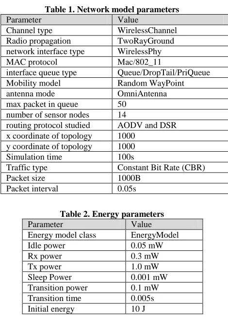
[image:2.595.313.548.70.396.2]The 1000 bytes constant bit rate traffic loads at 0.05s interval are transmitted during the simulation time. Other network parameters used in the simulation are shown in Table 1. Moreover, the parameters of energy model used in the simulation are presented in Table 2.
Table 1. Network model parameters
Value Parameter WirelessChannel Channel type TwoRayGround Radio propagation WirelessPhy network interface type
Mac/802_11 MAC protocol
Queue/DropTail/PriQueue interface queue type
Random WayPoint Mobility model
OmniAntenna antenna mode
50 max packet in queue
14 number of sensor nodes
AODV and DSR routing protocol studied
1000 x coordinate of topology
1000 y coordinate of topology
100s Simulation time
Constant Bit Rate (CBR) Traffic type
1000B Packet size
0.05s Packet interval
Table 2. Energy parameters
Value Parameter
EnergyModel Energy model class
0.05 mW Idle power 0.3 mW Rx power 1.0 mW Tx power 0.001 mW Sleep Power 0.1 mW Transition power 0.005s Transition time 10 J Initial energy
3.2
Simulation scenarios
The purpose of our work is to measure impact of mobility on performance of DSR and AODV routing protocols in terms of routing energy consumption, packet delay, and lost ratio. The findings lead the way to select more efficient routing protocol for the given WSNs each with different requirements. Therefore, to see the effect of mobility we need to compare the mobility results with the results when the sensor nods are stationary. To accomplish this, aside from the stationary scenario, four more distinct scenarios are designed by varying the number of hops in the route due to nodes mobility. The routes are established based on the AODV and DSR protocols which run separately in each scenario simulation. A description of the five scenarios is described as follows.
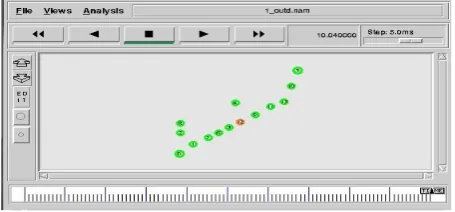
3.2.1 Scenario1: Stationary sensor nodes
Figure 1. WSN simulation envoronment in case of stationary sensor nodes
3.2.2 Scenario2: Mobile sensor nodes; increasing
number of hops
[image:3.595.316.545.74.216.2] [image:3.595.317.549.322.465.2]
The main goal in this scenario is to analyze performance of the protocols when mobility of the sensor nodes increases the length of the route. The sensor node12 changes its location to come between the main route (from node0 to node5). This will increase the number of intermediates nodes from 8 to 9. The simulation environment of this scenario is presented in Figure 2.
Figure 2. WSN simulation environment after increasing path length
3.2.3 Scenario3: Mobile sensor nodes; decreasing
number of hops
This scenario will focus on performance of the protocols when the established route is getting shorter due to the nodes mobility. The sensor nodes 6 and 13 change their locations to leave the main route. This results in decreasing the number of intermediates nodes from 8 to 6. The simulation environment of this scenario is presented in Figure 3.
Figure 3. WSN simulation envoronment after decreasing path length
3.2.4 Scenario4: Mobile sensor nodes; moving the
source sensor
[image:3.595.55.283.325.431.2]In this scenario node0 (source) moves and comes near to the
Figure 4. WSN simulation environment after moving source sensor
3.2.5 Scenario5: Mobile sensor nodes; moving the
destination sensor
Node5 (destination) moves to come near the node0 (source). The simulation environment of this scenario is presented in Figure 5.
Figure 5. WSN simulation environment after moving destination sensor
3.3 performance metrics
The major metrics to evaluate the scenarios are as follows.
a. Routing energy consumption level: is a function of the number and type of routing packets sent from the source to the destination for route discovery and maintenance. It is considered as energy required for the sum of all the routing control packets during transmission and reception between the source and destination. The energy consumption is analyzed to show the cost of each routing protocol with regard to energy.
b. End-to-End delay: it includes the average amount of time taken by a packet to go from the source sensor toward the destination sensor in WSN through a path made by the corresponding routing protocol.
c. Packet lost rate: it is the ratio of the number of packets sent by the source sensor to those received by the destination sensor node.
4.
SIMULATION RESULTS
[image:3.595.57.282.584.690.2]4.1 Experiment1
This experiment implements the scenario1 when all the sensor nodes are stationary. The results are presented as follows.
4.1.1 Routing energy consumption level
[image:4.595.56.284.169.326.2]The comparison of routing energy consumption when the sensor nodes are stationary is presented in Figure 5.
Figure 5. Energy consumption level for stationary sensor nodes
Based on the above results, when the nodes are stationary, during the entire simulation time, AODV consumes more energy than DSR. At the beginning of the simulation, both algorithms consume the highest amount of energy which is essentially required for the route discovery and making connection between the node0 and node5. After establishment of the connection, energy consumption decreases. Since the nodes are stationary, less routing traffic is required by DSR compared to AODV which performs frequent freshness checking. This is the reason of consuming more energy by the sensor nodes using AODV than DSR even after the connection establishment.
4.1.2 End-to-End delay
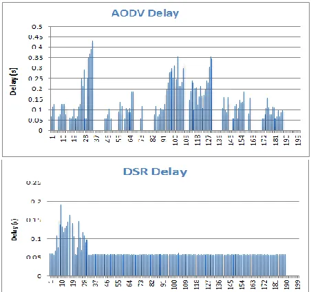
The delay comparison when the sensor nodes are stationary is presented in Figure 6.
Figure 6. Delay comparison for stationary sensor nodes
Based on the results, DSR is more efficient than AODV in term of less delay. DSR delay is lower and more stable than AODV. At the beginning of the route discovery, DSR delay increases. However, after the initial path discovery is done, DSR delay decreases and remains at the same level through the end of the simulation. In contrast, AODV shows more variations during the entire simulation time which is the result of frequent route checking. The gaps observed in the graph are the packets that lost due to the limited capacity of the buffer and also the packet buffering time exceeds the time limit.
4.1.3 Packet lost rate
[image:4.595.318.545.229.554.2]The comparison of packet lost rate when the sensor nodes are stationary is presented in Figure 7.
Figure 7. Packet lost comparison for stationary sensor nodes
When the nodes are stationary, AODV shows more packets lost than DSR. At the beginning of the simulation, DSR lost two packets due to the high number of routing traffics transmitted for the route discover. However, after that the number of lost packets for DSR is zero. In contrast, AODV shows loosing the packets during the entire simulation time even after the initial route discovery. This corresponds to the frequent discovery process as inherent characteristic of the AODV protocol.
4.2 Experiment2
[image:4.595.56.282.512.724.2]4.2.1 Routing energy consumption level
[image:5.595.56.283.123.244.2]The comparison of routing energy consumption when mobility results in increasing the number of hops is presented in Figure 8.
Figure 8. Energy consumption level comparison when path length increases
In this experiment, node12 moves toward the main route between node0 and node5. In this case although the number of hops increases in the path, still DSR shows less level of energy than AODV. Also DSR does not show a significant difference compared to the previous results when the nodes were stationary. The reason is that in DSR, the routes are maintained only between the nodes those want to communicate. Therefore, less routing traffic is required. Whereas, in AODV as the number of hops changes, the routing traffics to rebuild the new route increase which demands consumption of more energy. Thus, DSR is more efficient and consumes less energy.
4.2.2 End-to-End delay
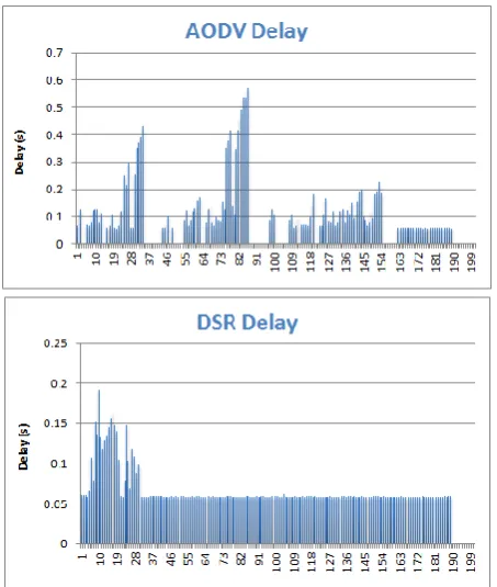
The comparison of delay when mobility increases the number of hops is presented in Figure 9.
Figure 9. Delay comparison when path length increases
quickly and shows similar delay variation as the previous experiment. However, delay is a little higher for AODV than before for a short time at the beginning. The reason is that while AODV is busy to make the initial path, after 1 second the node12 moves to come between the node0 and node5. So, new request and response routing packets must be exchanged to replace the older values which increase the delay. However, after that the delay decreases to almost the same amount as before.
4.2.3 Packet lost rate
[image:5.595.317.546.205.515.2]The comparison of packet lost rate when mobility increases the number of hops is presented in Figure 10.
Figure 10. Packet lost comparison when path length increases
The results in this experiment when the node12 moves and comes between the source (node0) and destination (node5) follow the same pattern like when the nodes are stationary. DSR just lost two packets since the beginning of the simulation. AODV performance in term of packet lost is less efficient than DSR and it loses many packets through the simulation run.
4.3 Experiment3
This experiment implements the scenario3 when the number of hops decreases as the sensor node3 and sensor node13 leave the main route. The results are presented as follows.
4.3.1 Routing energy consumption level
[image:5.595.56.283.459.727.2]Figure 11. Energy consumption level comparison when path length decreases
Based on the above results, energy consumption with AODV is more uniformly distributed over the network than the previous results as the number of hops decreases. In this experiment, the DSR caching mechanism makes less route discovery overhead than in AODV. This provides better performance for DSR than AODV.
4.3.2 End-to-End delay
The comparison of delay when mobility decreases the number of hops is presented in Figure 12.
Figure 12. Delay comparison when path length decreases
The result of this experiment shows that unlike the previous results, this time AODV works more efficient than DSR. The AODV still follows the same pattern but higher delay in compare to the previous experiments. However, under this new condition, DSR shows a completely different pattern than before. Unlike the previous experiments, DSR shows very high and instable delay distribution. The reason is that, after 1 second past, the node6 leaves the established route, so DSR
tries to discover new path. While DSR is busy to find new path, after 1 more second, node13 also leaves the path. So DSR delay increases highly and many packets collide resulting in packet lost and gaps in the graph.
4.3.3 Packet lost rate
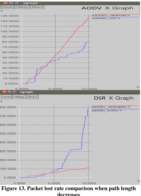
[image:6.595.318.545.184.500.2]The comparison of packet lost rate for AODV and DSR when mobility decreases the number of hops is presented in Figure 13.
Figure 13. Packet lost rate comparison when path length decreases
In this experiment DSR shows poor performance than AODV as it lost many packets due to changing the route between the source and destination. The higher rate of packet lost in compare to the number of received packets shows that DSR lost many packets during the route discovery after the node6 and node13 leaves the route. In this case, AODV shows better performance than DSR and lost less packet.
4.4 Experiment4
This experiment implements the scenario4 when after one second the source sensor (node0) comes closer to the destination sensor (node5). The results are presented as follows.
4.4.1 Routing energy consumption level
[image:6.595.55.283.389.653.2]Figure 14. Energy consumption level comparison when the source sensor moves
As the graph shows, both algorithms need the highest amount of energy to establish the initial path. When the source sensor moves to get closer to the destination sensor, AODV consumes more energy than DSR to make the new route to the destination. Also after that the entire simulation time shows that AODV still needs more energy than DSR.
4.4.2 End-to-End delay
The comparison of delay when mobility brings the source sensor closer to the destination sensor is presented in Figure 15.
Figure 15. Delay comparison when the source sensor moves
Based on the above results, making the initial route can cause more delay to the WSN with AODV protocol than DSR. Also after moving the source sensor, AODV still imposes more delay to establish the new path. After finding the final route,
4.4.3 Packet lost rate
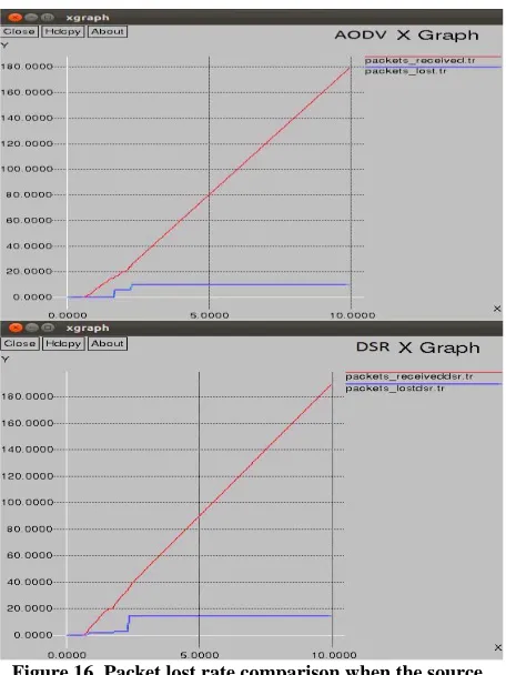
[image:7.595.317.545.135.439.2]The comparison of packet lost for AODV and DSR when the source sensor gets closer to the destination sensor, is presented in Figure 16.
Figure 16. Packet lost rate comparison when the source sensor moves
Based on the results AODV shows better performance than DSR in term of losing less packets. Both algorithms start losing the packets during establishing the initial path. Losing the packets by both algorithms also continues when the source sensor move and making a new path is required by the algorithms. However, after that losing the packets stop and the lost rate reaches zero.
4.5 Experiment5
This experiment implements the scenario5 when the destination sensor (node5) moves and comes closer to the source sensor (node0). The results are presented as follows.
4.5.1 Routing energy consumption level
[image:7.595.55.283.391.664.2]Figure 17. Energy consumption comparison level when the destination sensor moves
The results show that, the level of energy required by AODV to establish and maintain the route is higher than DSR. Comparing the above results with the Experiment4 shows that moving the source sensor consumes more energy by the both algorithms than moving the destination sensor.
4.5.2 End-to-End delay
The comparison of delay when mobility brings the source sensor closer to the destination sensor is presented in Figure 18.
Figure 18. Delay comparison when source sensor moves
The above results show a very high amount of delay for DSR when the destination sensor moves toward the source sensor. The results also show more gaps (lost packets) in the AODV graph. After finding the final route, the delay is stabilized in both graphs with smaller amount for AODV than DSR.
4.5.3 Packet lost rate
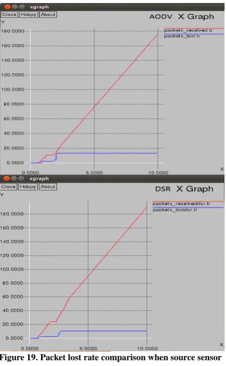
[image:8.595.317.545.136.505.2]The comparison of packet lost rate for AODV and DSR when the destination sensor moves to be near the source sensor is presented in Figure 19.
Figure 19. Packet lost rate comparison when source sensor
moves
The above results show poor performance of AODV in term of higher number of lost packets in compare to DSR to find the final route.
5.
CONCLUSION
In this study, performance comparison of DSR and AODV routing protocols for WSN was presented in terms of the energy consumption, delay, and lost ratio. From the results it can be concluded that DSR shows better performance than AODV when there is less mobility between the sensor nodes in WSN.
[image:8.595.56.283.369.641.2]6.
REFERENCES
[1] J. Jung, Y. Cho, and J. Hong. Impact of Mobility on Routing Energy Consumption in Mobile Sensor Networks, International Journal of Distributed Sensor Networks, Vol.2012, pp.1-12, 2012.
[2] K. Pandey and A. Swaroop. A Comprehensive Performance Analysis of Proactive, Reactive and Hybrid MANETs Routing Protocols, IJCSI International Journal of Computer Science, Vol. 8, No 3, 2011.
[3] S.S. Kumar, M.N. Kumar, V.S. Sheeba, and K.R. Kashwan. Evaluation of Hybrid Ad Hoc Routing Protocol for Wireless Sensor Network, Journal of Information & Computational Science, pp. 2107–2115, 2011.
[4] N. Kulkarni, R. Prasad, H. Cornean, and N. Gupta. Performance Evaluation of AODV, DSDV & DSR for Quasi Random Deployment of Sensor Nodes in Wireless Sensor Networks, International Conference on Devices and Communications (ICDeCom’11), pp.1-5, 2011.
[5] M. Barati, K. Atefi, F. Khosravi, and Y.A. Dafia. Performance Evaluation of Energy AODV and DSR Routing protocols in MANET, International Conference on Computer & Information Science (ICCIS’12), pp.1-7, 2012.
[6] R. Jain, N.B. Khairnar, and L.Shrivastava. Comparative Study of Three Mobile Ad-hoc Network Routing Protocols under Different Traffic Source, IEEE International Conference on Communication Systems and Network Technologies (CSNT), pp.104 – 107, 2011.
[7] V. Sahni, P.Sharma, J.Kaur, and S.singh. Scenario Based Analysis of AODV and DSR Protocols Under Mobility in Wireless Sensor Networks, International Conference on Advances in Mobile Network, Communication and Its Applications (MNCAPPS’12), pp.160 – 164, 2012.
[8] P. Goswami and A. D. Jadhav. Evaluating the Performance of Routing Protocols in Wireless Sensor Networks, IEEE International Conference on Computing Communication & Networking Technologies (ICCCNT), pp.1-4, 2012.
[9] A. A.S. Ihbeel, H. I. Sigiuk, and A.A. Alhnsh. Simulation Based Evaluation of MANET Routing Protocols for Static WSN, IEEE Second International Conference on Innovative Computing Technology (INTECH’12), pp.63 – 68, 2012.