Lossless Data Compression Using Rice Algorithm Based On Curve Fitting Technique

(1)

LOSSLESS DATA COMPRESSION USING RICE ALGORITHM BASED ON

CURVE FITTING TECHNIQUE

Ginu Thomas

1

_{, GK Sadanandan}

2

1

_{PG Student, ECE Department, Toc-H Institute of Science and Technology, Kochi, India}

2

_{Professor, ECE Department, Toc-H Institute of Science and Technology, Kochi, India}

---*---Abstract -**

Today, with the growing demands of information storage and data transfer, data compression is becoming greatly important. Data Compression is a technique which is used to decrease the size of original data. This is very useful when some huge files have to be transferred over networks or being stored on a data storage device. This project aims at the implementation of a lossless data compression system using the Rice algorithm using the mathematical curve fitting models. The Rice algorithm exploits a set of variable-length codes to achieve compression. This is done using a two-stage compressor, namely, a pre-processing two-stage followed by an adaptive entropy coder. A function is generatedbased on the input data sets that can be used to find points anywhere along the curve. A comparison between the data compression of modified Rice algorithm and ordinary Rice algorithm is also presented. The design can be implemented in VHDL using Modelsim.

Key Words: Fundamental sequence, Adaptive Entropy

Coder, Consultative Committee for Space Applications, Joint Photographic Experts Group

1.INTRODUCTION

The spread of computing has led to an explosion in the volume of data to be stored on hard disks and sent over the Internet. This growth has led to a need for data compression. Data compression is a process by which a file may be transformed to another file, such that the original file may be fully recovered from the original file without any loss of actual information. This process may be useful if one wants to save the storage space. For example if one wants to store a 4MB file, it may be preferable to first compress it to a smaller size to save the storage space. Also these compressed files are much more easily exchanged over the internet since they upload and download much faster. Data compression is a method of encoding rules that allows substantial reduction in the total number of bits to store or transmit a file. The more information being dealt with, the more it costs in terms of storage and transmission costs. In short, Data Compression is the process of encoding data to fewer bits than the original representation so that it takes less storage space and less transmission time while communicating over a network.

There are mainly lossless and lossy forms of data compression. A lossy data compression method is one where the data retrieves after decompression may not be exactly the same as that of original data. Some examples of lossy data compression algorithms are JPEG, MP3. Lossless data compression is a technique that allows the exact original data to be reconstructed from the compressed data. This is in contrary to the lossy data compression in which the exact original data cannot be reconstructed from the compressed data [8]. The Rice compression algorithm is one example of a lossless compression algorithm which is suitable for compression of certain types of data. This paper is based on a lossless data compression Rice Algorithm as recommended by the CCSDS for the reduction of required test data amount.

In this work we propose a strategy for designing optimum lossless data compression systems. In the following sections the algorithm is described, and then the modification of this algorithm is done. Simulation of both ordinary and modified algorithm and their comparison is done.

2. RICE ALGORITHM

The Rice algorithm uses a set of variable-length codes to achieve compression. Variable length coding is the compression method in which shorter code words are assigned to data that are expected to occur with higher frequency [4].

(2)

[image:2.595.36.285.97.346.2]

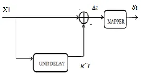
2.1 The Preprocessor

The preprocessing is done by using a unit delay followed by a prediction error mapper. The preprocessor is used to decorrelate data samples and subsequently map them into symbols suitable for the entropy coding stage [6].

2.1.1 Unit delay predictor

One of the simplest predictive coders is a linear first-order unit-delay which is shown in fig 2.1

Fig: 2..2 Unit Delay Predictor

The input data to the preprocessor, x, is a J-sample block of n-bit samples:

x = x1, x2, . . . xJ.

The output, Δi, will be the difference between the input data symbol and the preceding data sample.

2.1.2 Mapper

Based on the predicted value 𝑥𝑖 , the prediction error mapper converts each prediction error value, Δi, to an n-bit nonnegative integer, δi, suitable for processing by the entropy coder[5]. The

preprocessor transforms input data into blocks of preprocessed samples, δi, where:

δi = δ1, δ2, . . . δJ.

The prediction error mapping function is given by



= minimum (xiˆ– xmin, xmax – xiˆ)

[image:2.595.313.534.303.432.2]

Where Δi is the prediction error produced by the predictor, xmin and xmax denote the minimum and maximum values of any input sample xi.

Table 1.1 illustrates the operation of the prediction error mapper of 8-bit data samples of values from 0 to 255.

Sample value

x

_i

Predictor value xiˆ

Δi

_

i δi

38 - - - -

65 38 27 38 54

100 65 35 65 70

123 100 23 100 46

159 123 36 123 72

201 159 42 96 84

220 201 19 54 38

250 220 30 35 60

Table 1.1 Operation of Error Mapper

2.2 Adaptive Entropy Coder

The Adaptive Encoder converts preprocessed samples, δi, into an encoded bit sequence y. The entropy coding module is a collection of variable-length codes operating in parallel on blocks of J preprocessed samples. For each block, the coding option achieving the best compression is selected to encode the block. The encoded block is preceded by an ID bit pattern that identifies the coding option to the decoder.

The different compression options available are:  Fundamental sequence encoding  The split-sample options  Zero block option  No compression option

2.2.1 Fundamental Sequence Encoding

[image:2.595.86.232.513.591.2]

(3)

2.2.2 Split Sample option

[image:3.595.313.541.491.587.2]

Most of the options in the entropy coder are called 'split-sample options'. The kth split 'split-sample option takes a block of J preprocessed data samples, splits off the k least significant bits (LSB) from each sample and encodes the remaining higher order bits with a simple FS codeword before appending the split bits to the encoded FS data stream [6]. Table 2.1 shows some examples of split sample options.

Table 2.1: Example of Split Sample Options 2.2.3 Zero Block Option

The Zero-Block option is selected when one or more blocks of preprocessed samples are all zeros. In this case, the numbers of adjacent all zero preprocessed blocks are encoded by an FS code word.

2.2.4 No compression option

When none of the above options provides any data compression on a block, the no compression option is selected. Under this option, the preprocessed block of data is transmitted without alteration except for a prefixed identifier.

3. MODIFIED RICE ALGORITHM USING CURVE

FITTING TECHNIQUE

Curve fitting is the process of a curve or a mathematical function that best suits to a set of data points. An equation is produced by curve fitting that can be used to find points anywhere along the curve. Thus prediction of next data value (𝑥ˆ𝑖) is possible with this method [5]. It captures the trend in the data by assigning a single function across the entire range.

3.1 Polynomial Curve Fitting Method

The general form of a polynomial is given by









j k k k

x

a

x

f

1 0

)

(

The goal is to identify the coefficients

a

₀ and

a

_ksuch that f(x) fits the data well. Add up the length of data points and this gives the expression of the ‘error’ between data and fitted line. The curve that provides a minimum error is then the best curve, using least squares methodm[1]. The general expression for any error using the least squares approach is:

The best line has minimum error between line and data points. This is called the least squares approach, since we minimize the square of the error [1]. Substitute the form of eq. (2) into general least square error eq. (1), we get

Error=



 





j k k k n i

i

a

x

y

1 2 0 1

))

(

Where n-number of data points, i-current data point, j-order of the polynomial.

The best suited curve will give minimum error between line and data points. So the objective is to minimize the eq. (3) and also find the corresponding values of the coefficients

a

₀,

a

_k. To minimize eq. (3), take the derivative of error with respect to each coefficient

a

₀,

a

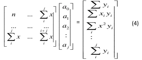
_kwhere k=1, 2….j, set each value to zero. Representing the equation using a matrix form as follows as:

             



j i i j i j i x x x n ... ... ... ... ...                 j a a a a : 2 1 0 =                      



j i i i i i i i y y x y x y : 2

To know the value of

a

₀,

a

_k,solve eq. (4).For that take

             



j i i j i j i x x x n ... ... ... ... ...                 j a a a a : 2 1 0 (1) (2) (3) (4)

(4)

        

 

        

 



j

i i i

i

y y x

y x

y

:

2

The following solution method can be used:

AX=B

Using built in Mathcad matrix inversion, the coefficients the values of coefficients a

a

₀,

a

_kare solved.

>> X = A1_*B

Finally a polynomial equation that fits for the data points is obtained. The coefficient values are then quantized; these values are then implemented in the function which is used to predict the next set of values [6].

4. SIMULATION RESULTS AND DISCUSSION

4.1 Rice Algorithm

The first stage is preprocessor which is used to decorrelate the input sample. The next data value is based on the current data value. The Table 4.1 shows the first sage output using ordinary Rice Algorithm.

Table 4.1 Output obtained during mapping using Rice algorithm

Fig. 4.1 Output waveform of Rice algorithm showing compressed data

Simulation result for Rice algorithm is shown in fig 4.1 using Modelsim. Here the 5thsplit sample option (byte7) is chosen as the minimum number of bits when compared with other options used, which is the compressed data.

4.2 Modified Rice Algorithm

[image:4.595.308.560.369.496.2]

In Modified Rice algorithm the next data value is obtained by using a curve fitting function based on the function generated, so that we can compress more data. The table 4.2 shows the output sage of preprocessor in modified Rice algorithm.

Table 4.2: Output obtained during mapping using modified Rice algorithm

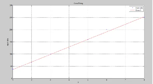
Fig 4.2 Curve fitted values obtained using modified RICE algorithm in Matlab.

[image:4.595.38.282.481.546.2]

The next data values obtained during mapping using modified rice algorithm is shown in fig 4.2. Function values are obtained through curve fitting method using Matlab.

Fig 4.3 Simulation result in Matlab: Graph showing 8 input samples and curve fitting function

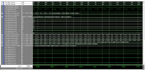
[image:4.595.309.560.590.729.2] [image:4.595.37.288.596.726.2]

(5)

[image:5.595.36.288.109.231.2]

modified rice algorithm showing compressed data

Here the 2ndsplit sample option (byte4) is chosen as the minimum number of bits when compared with other options used, which is the compressed data.

For the above example the number of bits in compressed data is 30 (Fig 4.4) when modified rice algorithm is used. Whereas the number of bits in compressed data is 52 (Fig: 4.1) when modified rice algorithm is used. Thus the number of bits of compressed data reduces when modified rice algorithm is used.

4. COMPARISON BETWEEN RICE ALGORITHM

AND MODIFIED RICE ALGORITHM

1. In rice algorithm, we predict that the next data which is similar to that of the current data. Whereas in modified rice algorithm based on curve fitting, a function is developed for the given set of inputs [5] and so the next data value can be predicted according to the function which results in smaller δ values. Hence we can compress more data.

2. Higher compression is possible when modified Rice algorithm is applied to a set of inputs.

3. In rice algorithm, after compression while sending the data to the receiver, a reference, (n-1) values of δ and the ID corresponding to the compression option used are transmitted. Whereas in modified rice algorithm the function coefficients, n values of δ and the ID corresponding to the compression option are transmitted to the receiver.

5. CONCLUSIONS

In this paper, a comparison between the Rice algorithm and modified Rice algorithm is done. The basic idea behind Rice coding is to store as many words as possible with less bits than in the original representation o that we can reduce the storage volume. In the case of ordinary Rice algorithm, the next data value is based on the current data value but in the case of modified rice algorithm with curve fitting, a function is generated based on the input data set, with which upcoming values are predicted. These

predicted values will be small and hence we can compress more data’s as compared to ordinary Rice algorithm. Thus later method finds numerous applications in most of the industries especially in space applications. The simulation result shows that the data is compressed more with modified rice algorithm.

REFERENCES

[1] Gurley, Numerical Methods Lecture 5 - Curve Fitting

Techniques, Computer Methods

[2] Armein Z. R. Langi, “An FPGA Implementation of a

Simple Lossless Data Compression Coprocessor”, IEEE,

17-19 July 2011

[3] CCSDS (Consultative committee for space data systems),

GREEN BOOK ISSUE-2, December 2006

[4] R. F. Rice and J. R. Plaunt, “Adaptive variable length

coding for efficient compression of spacecraft television

data,” IEEE Trans. Commun. Techno.Vol. COM-19, part I,

pp. 889-897, Dec. 1971.

[5] Pratheeka Paulose, “Implementation Of Modified Rice

Algorithm Based On Curve Fitting Techniques”, International Journal of Advanced Research in Electrical, Electronics and Instrumentation Engineering, Vol. 2, Issue 6, June 2013

[6] Rakhee Sasi, “CCSDS Lossless Data Compression

Algorithm in FPGA for Space Applications” International

Journal of Engineering and Advanced Technology, Volume-2, pp: 2249 – 8958 ,Issue-6, August 2013

[7] Salvatore Coco, Valentina D’Arrigo, Domenico Giunta, “A

Rice-Based Lossless Data Compression System For Space Applications”, pp. 377-381, July 2015

[8] Amarjit Kaur, “A Review on Data Compression

Techniques”, IJARCSSE, Volume 5, Issue 1, January 2015

[9] Udaya Kumar H, Madhu B C, “Design and

Implementation of Lossless Data Compression

Coprocessor using FPGA”, IJERT, Vol. 4 Issue 05,

Lossless Data Compression Using Rice Algorithm Based On Curve Fitting Technique