Determining Microscopic Traffic Variables using
Video Image Processing
Abdulrazzaq Alkherre
t
Graduate Ph.D Student
Faculty of Engineering Cairo University, Egypt
Al-Sayed A. Al-Sobky
Assistant Professor
Faculty of Engineering Ain Shams Univ., Egypt
Ragab M. Mousa
Professor
Faculty of Engineering Cairo University, Egypt
ABSTRACT
Vehicle detection and tracking play an important role in traffic management and control. Among available techniques, Video Image Processing (VIP) is considered superior due to ease in installation, maintenance, upgrade, and visualizing results while processing recorded videos. In this paper, a multiple-vehicle surveillance model was developed, using Matlab programming language, for detecting and tracking moving vehicles as well as collecting traffic data such as traffic count, speed, and headways. The developed model was validated for different lengths of region of interest (ROI), ranging between 5 and 30 m. Validation was established using simulated video clips, designed in VISSIM, and traffic data obtained from model were compared with actual measurements reported by VISSIM. Vehicle counts (or detections) obtained from the model are identical to actual counts. Comparison of speeds confirmed the model validity, especially with 10 m and 15 m ROI lengths. For these lengths, the mean difference of speeds is not significant at 5% significance level. Validation headway measurements was also confirmed for ROI of 10 and 15 m. With such successful validation, the model features many applications. Beside traffic data collection, the model can be applied for incident detection, speed enforcement, intelligent transportation system, etc. However, the model was validated assuming no lane changes. Camera position was also set to avoid overlap of vehicles. Accordingly, the model validity is limited to these assumptions. Further research is currently in progress to extend model validity to lane changes and different camera positions.
Keywords
Matlab, Image Processing, Traffic Surveillance, Vehicle Detection, Vehicle Tracking, Speed, Headway.
1.
INTRODUCTION
The literature is abundant with researches that dealt with detection and tracking of moving objects in video sequence, and numerous mathematical models have resulted out of these studies. A general subdivision of object detection techniques can be made of three main categories, namely, (a) Background Subtraction, (b) Temporal Differencing, and (c) Optical Flow. Similarly, the object tracking can be divided into three main categories, Point tracking, Kernel tracking, and Silhouette tracking [1].
In object detection techniques, Background Modeling (Background Subtraction) is used to detect moving objects in an image by taking the variations between the current image and the reference background image in a pixel-by-pixel fashion. The background subtraction method uses a simple
algorithm. However, it is very sensitive to changes in the external environment. Similarly, Temporal Differencing method is used to calculate the absolute differences between two consecutive images to extract moving regions and obtain a threshold function to determine changes. The temporal differencing has a strong adaptability for a variety of dynamic environments, but its method of calculation is generally difficult to achieve complete outline of moving object. The Optical Flow method uses the optical flow distribution characteristics of moving objects over time in an image sequence. Flow computation methods cannot be applied to video streams in real time because they are very complex and very sensitive to noise [2] and [3].
In object tracking manners, the Point tracking method is based on monitoring and comparing the positions of different detected points from one frame to another. Kernel tracking method tracks objects by calculating the motion of an object shape and its appearance in successive frames. The Silhouette tracking method uses information inside the silhouette's region in the form of edged maps to track the object using shape matching approach [4] and [5].
As mentioned above, background subtraction methods are very sensitive to changes in the scene. Also, this method requires a training period absent of foreground objects and too slow to be practical. Stauffer and Grimson [6] modeled each pixel in an image sequence as a mixture of Gaussians and used an on-line approximation to update the model. Then, the Gaussian distributions of the adaptive mixture model are evaluated to determine which are most likely to result from a background process. Finally, each pixel is classified based on whether the Gaussian distribution which represents it most effectively is considered part of the background model. Kaewtrakulpong and Bowden [7] improved the previous adaptive background mixture model. The authors updated equations and utilized different equations at different phases to make their system learn faster and more accurately as well as adapt effectively to changing environments. However, Matlab [8] adopted the previous two studies and presented a System object to detect foreground using Gaussian Mixture Models (GMMs).
systems are capable of supporting multiple lane and multiple detection zone applications. In comparison to all other technologies, VIP system is considered the best in terms of installation, maintenance and portability improvement. Moreover, this technology allows users to check visually the results by watching videos previously recorded.
A VIP system typically consists of one or more cameras, a microprocessor-based computer for digitizing and analyzing the imagery, and software for analyzing the imagery of traffic stream to determine changes between successive frames and converting them into traffic flow data [12] and [13].
The review of the literature revealed the lack of studies dealing with the impact of vehicle detection zone (ROI) on the accuracy of detections and measured speeds of individual vehicles. Furthermore, most reviewed studies focused only on speed as the prime traffic data.
It is, therefore, the objective of this research to collect traffic data of detected vehicles and assess the impact of the size of ROI on the accuracy of such collected data. This paper presents the development of a multiple-vehicle surveillance model based on the features of Matlab programming language, especially the image processing toolbox. A Video-Based Detection And Tracking Model called "VBDATM" was developed in the course of this research. The paper also summarizes the main findings of the model applications, features, and limitations.
2.
DEVELOPMENT OF THE PROPOSED
MODEL
This section presents the efforts devoted in developing the proposed model. The proposed model is developed using Matlab Programming Language and consists of three sequential modules, namely, Detection, Tracking, and Traffic Data Collection as outlined below.
Detection Module: in this module, the moving vehicle is detected as it enters the ROI and exact time and location are registered while vehicle is traveling in the ROI. This is repeated in each frame until the vehicle leaves ROI. These steps are repeated for all vehicles in the video clip. Tracking Module: in this module, data of detected
vehicles recorded in frames are checked to segregate all frames belonging to each vehicle and storing them in a separate sheet. This data is simply spatial and temporal data of vehicle trajectory while traveling in the ROI. Each data sheet belongs to only one vehicle.
Traffic Data Collection Module: With the availability of spatial and temporal data of each vehicle, traffic data such as flow, speed, headway, and possibly density can be computed in this module.
The methodology executed in each module is discussed in some detail in the following sections.
2.1.
Vehicle Detection Methodology
Vehicle detection is the first step prior to performing more sophisticated tasks such as tracking [8]. In this paper, an interactive code was written to detect and track moving vehicles in video sequence using foreground detection based on Gaussian Mixture Models. The code for detection consists of three main parts; initialization, external functions, and stream processing loop. These are elaborated in the following
2.1.1.
Initialization
The reason for initialization at the beginning of this module is to:
- Read the video from *.avi file,
- Read and store the height and length of video frames and frame rate,
- Display the first frame of the video clip,
- Read the limits of the region of interest (ROI) and lane separators as interactively defined by the user on the screen using the mouse.
- Assign variables to store the coordinates of these limits and the length of the region in pixel.
- Read the length of the ROI in meter. This step is performed to create a Conversion Factor which is used to convert dimensions in pixels to meters and vice versa.
- Read the expected maximum speed (km/h). The Conversion Factor and the maximum speed are used to calculate the maximum distance that a vehicle can travel in single frame (step/frame).
2.1.2.
External Functions
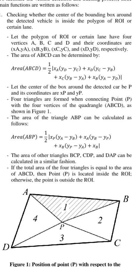
To facilitate the vehicle detection and tracking process, three main functions are written as follows:
1. Checking whether the center of the bounding box around the detected vehicle is inside the polygon of ROI or certain lane.
- Let the polygon of ROI or certain lane have four vertices A, B, C and D and their coordinates are (xA,yA), (xB,yB), (xC,yC), and (xD,yD), respectively. - The area of ABCD can be determined by:
- Let the center of the box around the detected car be P and its coordinates are xP and yP.
- Four triangles are formed when connecting Point (P) with the four vertices of the quadrangle (ABCD), as shown in Figure 1.
- The area of the triangle ABP can be calculated as follows:
- The area of other triangles BCP, CDP, and DAP can be calculated in a similar fashion.
[image:2.595.319.542.303.752.2]2. Calculating the travel distance between two given frames. The distance traveled by a vehicle (∆D) during two frames is calculated using the following formula:
Where (x1, y1) are the coordinates of the vehicle center in 1st frame, and (x2, y2) are the coordinates in 2nd frame. 3. Calculate the vehicle travel distance inside the ROI.
- Let the current position of a detected vehicle be at Point P (xP, yP) and the start line of ROI is at Line BC connecting the two points B (xB, yB) and C (xC, yC) as indicated in Figure 1.
- The slope (m) of the line BC is given by:
- The travel distance (TD) can be calculated as the perpendicular distance from the vehicle position to the start line of ROI. The travel distance (TD) can be calculated as follows:
2.1.3.
Stream Processing Loop
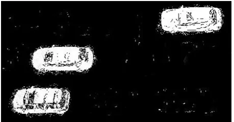
The main purpose of this loop in detection process is to detect the vehicles in the input video. The processing loop uses the variables created in the initialization stage and the external functions mentioned above. The loop includes three stages. Stage 1 reads the input video frame and detects the foreground. Foreground detection means converting the colored frame, as shown in Figure 2-a, to a binary image (black and white image) with the same dimensions based on a conversation threshold. Black areas refer to the fixed background of the scene whereas white areas (blobs) refer to the moving objects, as shown in Figure 2-b.
The foreground segmentation process does not produce perfect moving objects and often includes undesirable noise due to the use of improper conversation threshold. In Stage 2, the noise is removed from the foreground image using special morphological filters and another proper binary image is produced as shown in Figure 2-c.
Stage 3 begins by estimating the bounding box around every blob in the foreground image and then the center coordinates of each box can be estimated as shown in Figure 3. Using the External Functions 1 and 2, the lane number and travel distance inside ROI can be determined.
[image:3.595.317.547.71.191.2]Figure 2-a: The original video image
[image:3.595.318.546.242.363.2]Figure 2-b: The image after foreground segmentation stage
[image:3.595.318.547.406.526.2]Figure 2-c: The image after noise removing stage
Figure 3: The image after establishing bounding boxes around detected vehicles
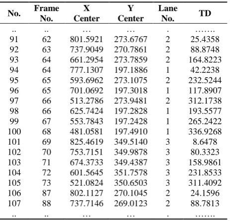
[image:3.595.54.285.583.712.2]Finally, the frame number, X-center, Y-center, travel distance, and lane number are stored in “Frame-by-Frame” array. For simplicity, this frame is referred to as FBF Array. Effective frames are only those frames of vehicles inside the ROI. The “FBF” Array is the major output of the vehicle detection process. Table 1 shows an example of this output.
Table 1: An example of detection data stored in “FBF” array
No. Frame No. X Center Y Center Lane
No. TD
.. .. … … . …….
91 62 801.5921 273.6767 2 25.4358 92 63 737.9049 270.7861 2 88.8748 93 64 661.2954 273.7859 2 164.8223 94 64 777.1307 197.1886 1 42.2238 95 65 593.6962 273.1075 2 232.5244 96 65 701.0692 197.3018 1 117.8907 97 66 513.2786 273.9481 2 312.1738 98 66 625.7424 197.2828 1 193.5577 99 67 553.7843 197.2428 1 265.2422 100 68 481.0581 197.4910 1 336.9268 101 69 825.4619 349.5140 3 8.6478 102 70 753.7151 349.9878 3 80.3323 103 71 674.3733 349.4387 3 158.9861 104 72 601.5645 351.7578 3 231.8533 105 73 521.0824 350.6503 3 311.4092 106 87 802.1127 270.1045 2 24.1596 107 88 737.7146 269.0123 2 88.7813
.. .. … … . …….
2.2.
Vehicle Tracking Methodology
In its simplest form, the vehicle tracking aims to keep track of already detected vehicles and isolate data of each vehicle. Vehicle tracking process move rows in FBF Array that belong to the same vehicle to a separate sheet or array called "VEH" Array. The flow diagram shown in Figure 4 illustrates the main steps executed during the tracking process. As shown in this figure, a three dimensional array VEH (r, 5, NVEH) is declared at the beginning of this process, where (r) is the maximum number of frames that belong to any vehicle, and NVEH is the number of pages, which is equal to the number of vehicles processed in the video, i.e., each page is dedicated to only one vehicle.
At the beginning of the tracking process, the first row in the “FBF” Array is copied to the first row of the first page of the "VEH" Array. This record is considered a reference or “REF” for simplicity. The rest of rows in FBF Array are compared individually with this “REF” in the first page. The comparison includes frame numbers, the travel distance between the two frames, the travel lane, and the travel distances for the two frames inside the ROI. The comparison of the row (or frame) inni noutq uq“FBF” Array and the “REF” row (frame) in certain page fails if at least one of the following conditions is not satisfied:
- Frame numbers are not equal,
- The distance between the two centers is less than the preset “Max-Step”,
- The travel lane is the same for both frames, and
- The travel distance inside ROI of the row (or frame) in question in Array “FBF” is greater than that of the “REF” row (or frame).
If the comparison fails, then the row (frame) in question is copied to a new page and used as the “REF” for that page. On the other hand, in case all conditions are met, it is copied at the bottom of current page and considered a new “REF” for the same matched page or vehicle.
resulting for one vehicle is shown in Table 2, which indicates that the vehicle was traveling in lane No. 2 and entered the ROI in Frame No. 62 and left it in Frame No. 66. The last column shows the location of this vehicle (in pixels), measured from the start of ROI.
Table 2: Example of one vehicle tracking data stored in “VEH” array
No. Frame
No. X Center (pixels) Y Center (pixels) Lane No. Distance (pixels)
91 62 801.5921 273.6767 2 25.4358 92 63 737.9049 270.7861 2 88.8748 93 64 661.2954 273.7859 2 164.8223 95 65 593.6962 273.1075 2 232.5244 97 66 513.2786 273.9481 2 312.1738
2.3.
Traffic Data Collection Module
This module utilizes the proposed model in acquiring traffic data from the detected and tracked vehicles. Types of data that can be collected by the proposed model are discussed in the following sections.
2.3.1.
Calculation of Spot Speed in the ROI
Estimating a vehicle speed mainly depends on the data stored in “VEH” Array for such vehicle. The coordinates of the center point are used to measure the travel distance inside ROI in pixels, then the conversion factor is used to convert this distance into meters. Similarly, differences in the frames numbers determine the travel time inside ROI in terms of frames. The frame rate of video is then used to convert the travel time into seconds. For example, using Table 2, the total travel distance (∆D) is:
The total travel time (TT ) = Leaving frame – Entry frame = 4 frames
Assuming that the conversion factor = 0.022 (m/pixel), and frame rate = 10 frame/second, the vehicle speed can be calculated as:
or
V = 57.1 km/h.
2.3.2.
Calculation of Headways in the ROI
The headway between two successive vehicles traveling in the same lane can be determined since time of the entry frame to ROI is recorded for each vehicle. Referring to Table 1, the first vehicle entered ROI in Lane no. 2 in Frame no. 62 and the next vehicle entered the same lane in Frame 87. The headway can then be calculated using the video frame rate as follows:
2.3.3.
Calculations of Other Traffic Data
Other traffic data can be obtained. As such, vehicle count can be taken the same as the number of detections or headways in each lane. This traffic count can be used to calculate the traffic flow rate (Q) in vph. Average traffic speed (V) can also be computed from speeds of individual vehicles measured in the ROI. The gaps between successive vehicles can also be computed by multiplying the headway between the two vehicles and the speed of the lag vehicle. The average traffic density (K) can be computed as Q/V in veh/km.
3.
VALIDATION OF THE DEVELOPED
MODEL
This section presents the validation of the proposed model using data obtained from the traffic simulation software (PTV VISSIM 6). The reasons for using simulation for validation include; (a) difficulty in obtaining permits in Cairo City to record video films with the required specifications and clarity, and (b) VISSIM can report the exact time and speed of each vehicle when it crosses certain screen line or data collection station. This feature eliminates the possibility of human errors in case data is extracted manually from played video clips.
3.1.
Preparation of Video Clips for use in
Validation
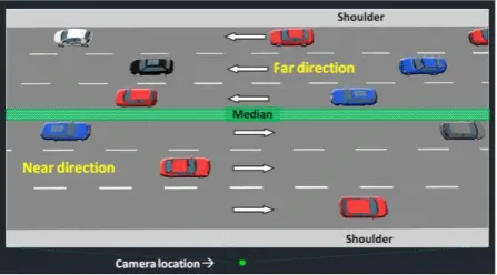
Higher mounting position allows for better angle and wider view, covering all lanes on the road by one camera. On the contrary, lower mounting heights would not provide effective images as some vehicles may hide part of other vehicles from the scene [13]. As a result, video image processing recognizes overlapped vehicles as a single object. Due to this fact, camera locations have been selected to provide sufficient field of vision and prevent overlapping of vehicles. The camera height was set to 30 m with 1 m lateral offset, and 65° pitch angle.
[image:6.595.315.539.147.262.2]A 6-lane divided highway with 3.5 m lane width was created in VISSIM and traffic was simulated for 330 sec. Figure 5 shows the layout of this road section and the directions (far or near) with respect to the camera location. Lanes in each direction are labeled shoulder lane, middle lane, and median lane.
Figure 5: Layout of road section considered in VISSIM for producing video clips
Before the start of simulation, a section of 30 m long was considered for data collection. In particular, 13 lines were drawn across the 6 lanes at 2.5 m intervals. The total distance between the first and last lines is 30 m. The intersection points
[image:6.595.59.283.509.633.2]of these lines with each lane give 13 stations for data collection along each lane. This makes a total of 78 data collection stations (or points) in the 6 lanes. Numbering and arrangements of these stations across the 6 lanes and lines are shown in Figure 6.
Figure 6: Locations of the 78 data collection points across the 6 lanes
At the end of simulation, VISSIM creates two files in AVI and text formats. The AVI file contains the video clip of simulated traffic motion and the text one contains the speed and the passing time of each vehicle at data collection points (or stations).
3.2.
Running the Developed Model for Data
Collection
In Matlab environment, the developed model was utilized to analyze the video clip (VISSIM AVI format file) for different lengths of ROI, namely, 5, 10, 15, 20, 25 and 30 m. For each ROI length, the model was set up to detect, track, and collect traffic data for the specified ROI length. These data are then compared with their counterparts produced by VISSAM (actual traffic data). As such, when the 5 m ROI is used, the model was run considering the ROI equal to area between the first and third lines marked in the video clip. The traffic data obtained for shoulder lane (Far direction) from the model are compared with the average data obtained from VISSIM at collection Points no. 1, 2, and 3 (refer to Fig. 6). Similarly, when the 30 m ROI is used, the collected data using the model for the same lane are compared with the average data obtain from VISSIM at collection Stations (points) no. 1, 7, and 13, and so on.
3.3.
Comparative Analysis of Model Results
The developed model was run 6 times to detect and track moving vehicles in the video clip for 6 different lengths of the region of interest (ROI). Results obtained from the model are compared with their counterparts obtained from VISSIM. This comparison is presented in the following sections.
3.3.1.
Comparison of Traffic Counts
Table 3: Number of vehicles counted (detected) by the Model
ROI Length
Near-Direction Far-Direction
Shoulder Middle Median Shoulder Middle Median Total
Lane Lane Lane Lane Lane Lane
5 m 124 123 123 115 112 115 370
10 m 124 123 123 115 112 115 370
15 m 124 123 123 115 112 115 370
20 m 124 123 123 115 112 115 370
25 m 124 123 123 115 112 115 370
30 m 124 123 123 115 112 115 370
Total 744 738 738 690 672 690 2220
3.3.2.
Comparison of Vehicles Speed
A comparative analysis was established between the vehicles speed collected by the developed model and the actual speeds reported by VISSIM for the six lengths of ROI mentioned above. The main objective of this analysis is to test whether not the proposed model can produce accurate speeds that are close to actual values. This check was made in three steps. First, the check was made visually by inspecting graphs showing values
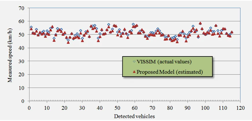
obtained from model and actual values. As an example, Figure 7 depicts a comparison between speeds obtained from the model and actual speeds for the shoulder lane of the Far direction when ROI of 10 m is used. The figure clearly shows that the speed resulted from the model is very close to the actual speed (produced by VISSIM). This close pattern is applicable for all lanes and for all ROI lengths.
Figure 7: Comparison of speeds obtained from model and actual speeds
The second step of comparison was made by computing the mean and standard deviation of the speeds obtained from model and actual speeds. The accuracy of the model estimates was expressed as the ratio of the mean speed of model and mean speed of actual values. The ratio of standard deviations was also computed. These results are shown in Tables 4 and 5 for speed and standard deviation, respectively.
As shown in Table 4, the mean speed obtained from model is very close to that of actual speed, typically, the ratio ranges between 96.7% and 99.5%. Notable comments can made on the ratios shown in this table; (a) model values are slightly less than
the actual values, (b) accuracy of model results is relatively high for Near direction than for Far direction, and the best model accuracy is associated with ROI lengths of 10 and 15 m. The standard deviation results shown in Table 5 indicate that all ratios are greater than 1.0. This means that the developed model produces relatively higher variation in individual speeds compared with the actual speeds. Furthermore, this variation is higher for Far direction lanes than for Near direction lanes. In addition, the least variation is reported with the ROI lengths of 10 and 15 m compared with other ROI lengths.
[image:7.595.80.516.339.549.2]Table 4: Ratio of mean speed from model and actual speed
ROI Length
Far-Direction Near-Direction
Shoulder Middle Median Shoulder Middle Median
Lane Lane Lane Lane Lane Lane
5 m 98.5 98.8 97.8 97.7 97.8 97.5
10 m 99.5 99.5 99.5 99.0 99.0 99.1
15 m 99.4 99.3 99.4 98.9 99.0 99.4
20 m 98.3 98.6 98.3 98.2 98.0 98.4
25 m 98.7 98.6 99.2 98.3 97.7 98.4
30 m 98.8 97.8 98.2 96.7 97.4 96.9
[image:8.595.100.498.246.353.2]Average 98.9 98.8 98.7 98.2 98.2 98.3
Table 5: Ratio of standard deviation of model speed and actual mean speed
ROI Length
Near-Direction Far-Direction
Shoulder Middle Median Shoulder Middle Median
Lane Lane Lane Lane Lane Lane
5 m 1.12 1.17 1.34 1.36 1.45 1.57
10 m 1.05 1.02 1.03 1.07 1.15 1.04
15 m 1.02 1.01 1.00 1.09 1.16 1.14
20 m 1.14 1.11 1.16 1.29 1.37 1.39
25 m 1.13 1.16 1.16 1.35 1.26 1.41
30 m 1.25 1.34 1.31 1.35 1.50 1.44
Average 1.12 1.13 1.17 1.25 1.31 1.33
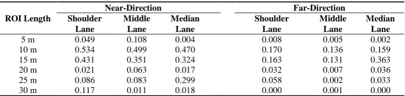
The third step in comparison to conclude the model validation is to perform a t-test on the two data sets for each ROI case. Before conducting this test, however, the Kolmogorov-Smirnov test was performed on the data sets to check whether
[image:8.595.92.505.445.543.2]observations of each data set are normally distributed. SPSS-V20 [14] was used to perform this test and results confirmed that all data are normally distributed. Results of the T-tests are shown in Table 6 for different lanes and ROI lengths.
Table 6: T-test results for comparison of model and actual speeds (P-value)
ROI Length
Near-Direction Far-Direction
Shoulder Middle Median Shoulder Middle Median
Lane Lane Lane Lane Lane Lane
5 m 0.049 0.108 0.004 0.008 0.005 0.002
10 m 0.534 0.499 0.470 0.170 0.136 0.159
15 m 0.431 0.351 0.324 0.163 0.131 0.363
20 m 0.021 0.063 0.017 0.032 0.007 0.036
25 m 0.086 0.083 0.299 0.058 0.002 0.033
30 m 0.117 0.011 0.018 0.000 0.001 0.000
As shown in this table, P-values less than 0.05 indicate significant difference between the model and actual speeds whereas greater values confirm that the difference between the model and actual speeds is not significant at the 5% significance level. Based on the results of this test, it can be concluded that the model produces speeds that are not significantly different from actual speeds for ROI lengths of 10 and 15 m, and this is valid for all 6 lanes. Accordingly, it can be concluded that the proposed model is valid for use with ROI length of 10 m or 15 m. It is interesting to note that although the model produces speeds with mean speed close to actual mean speed (> 96.5% ) for ROI of 5, 20, 25, and 30 m, the difference between the two means was significant.
3.3.3.
Comparison of Measured Headways
Measuring the individual headways (or gaps) between successive vehicles is essential because they indicate how
vehicles are dispersed and whether they follow too close from each other. Measuring headways can help in assessment of safety conditions on the road. Furthermore, the number of headways measured for certain time is a direct measure of the traffic flow. Furthermore, with average speed (V) and average flow (Q) available, one can readily calculate the average flow density (K) as the subdivision of Q and V (or K=Q/V).
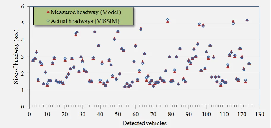
Figure 8: Comparison of headways obtained from model and VISSIM
Table 7: Results of T-tests for comparison of model headways
ROI Length
Near-Direction Far-Direction
Shoulder Middle Median Shoulder Middle Median
Lane Lane Lane Lane Lane Lane
10 m 0.9996 0.9995 0.9990 0.9906 0.9992 0.9980
15 m 0.9952 0.9913 0.9952 0.9934 0.9924 0.9980
4.
CONCLUSIONS AND
RECOMMENDATIONS
This paper presents a multiple-vehicle surveillance model, written in Matlab programming language, for vehicle detection, tracking, and collection of traffic data. The model was validated by processing video clips created in VISSIM. Based on the analysis presented in this paper, it can be concluded that the proposed model is a valuable tool for collecting essential traffic data such as speed, flow, and headways, which can save time and resources. The model produces its best results with optimum ROI lengths, namely, 10 and 15 mm. As expected, the accuracy of model results for the Near direction lanes are relatively better than those of lanes in the Far direction. The model can also be utilized in more advanced applications such incident detection, speed enforcement, intelligent transportation system, traffic control, etc. However, the model was validated using video clips of simulated traffic streams. No lane changes were assumed to occur near the ROI and camera position was selected so as to avoid any overlap between adjacent vehicles. Accordingly, the model applications might be limited to such assumptions. Further research is currently in progress to extend the model validity to video clips having lane changes and different camera positions.
5.
REFERENCES
[1] Parekh H. S., Thakore D. G, Jaliya U. K. 2014. A Survey on Object Detection and Tracking Methods. International Journal of Innovative Research in Computer and Communication Engineering (IJIRCCE). Vol. 2, Issue 2, February.
[2] Athanesious J. J., and Suresh P. 2012. Systematic Survey on Object Tracking Methods in Video, International Journal of Advanced Research in Computer Engineering & Technology (IJARCET) October, 242-247.
[3] Kastrinaki V., Zervakis M., Kalaitzakis K. 2003. A survey of video processing techniques for traffic applications. Image and Vision Computing 21: 359–381.
[4] Yilmaz A., Javed O., and Shah M. 2006. Object tracking: A survey. ACM Computing Surveys, 38:266-280, December.
[5] Hu W., Tan T., Wang L., and Maybank S. A. 2004. Survey on Visual Surveillance of Object Motion and Behaviors. IEEE Transactions on Systems, Man, and Cybernetics— Part C: Applications and Reviews, Vol. 34, No. 3, August. [6] Stauffer C., and Grimson W. E. L. 1999. Adaptive
[image:9.595.91.505.357.441.2][7] Kaewtrakulpong P., Bowden R. 2001. An Improved Adaptive Background Mixture Model for Realtime Tracking with Shadow Detection, In Proc. 2nd European Workshop on Advanced Video Based Surveillance Systems, AVBS01, Video Based Surveillance Systems: Computer Vision and Distributed Processing.
[8] MATLAB User’s Guide. 2012. MathWorks. www.mathworks.com.
[9] Klein L. A., Mills M. K., and Gibson D. R. P. 2006. Traffic Detector Handbook. Third Edition-Volume I. Turner-Fairbank Highway Research Center, McLean, VA. [10]Martin, P. T, Feng Y., and Wang X. 2003. Detector
Technology Evaluation. Publication UT-03.30. Utah Department of Transportation, Salt Lake City, UT.
[11]Klein L. A. 2001. Sensor Technology and Data Requirements for ITS. Artech House, Boston.
[12]Leduc G. 2008. Road Traffic Data: Collection Methods and Applications. Institute for Prospective Technological Studies.
[13]Mimbela L. E. Y, Klein L. A, Kent P., Hamrick J. L, Luces K. M, and Herrera S. 2007. A Summary of Vehicle Detection and Surveillance Technologies Used in Intelligent Transportation Systems. FHWA Intelligent Transportation Systems Program Office.