Heavy Tailed Distributions Generated by Randomly Sampled Gaussian, Exponential and Power Law Functions

(1)

http://dx.doi.org/10.4236/am.2014.513198

Heavy-Tailed Distributions Generated by

Randomly Sampled Gaussian, Exponential

and Power-Law Functions

Frederic von Wegner

Medical Biophysics Group, Institute of Physiology and Pathophysiology, University of Heidelberg, Heidelberg, Germany

Email: [email protected]

This work is licensed under the Creative Commons Attribution International License (CC BY).

http://creativecommons.org/licenses/by/4.0/

Abstract

A simple stochastic mechanism that produces exact and approximate power-law distributions is presented. The model considers radially symmetric Gaussian, exponential and power-law func- tions in n = 1, 2, 3 dimensions. Randomly sampling these functions with a radially uniform sam- pling scheme produces heavy-tailed distributions. For two-dimensional Gaussians and one-dimen- sional exponential functions, exact power-laws with exponent −1 are obtained. In other cases, densities with an approximate power-law behaviour close to the origin arise. These densities are analyzed using Padé approximants in order to show the approximate power-law behaviour. If the sampled function itself follows a power-law with exponent −α, random sampling leads to densities that also follow an exact power-law, with exponent n 1

α

− − . The presented mechanism shows that power-laws can arise in generic situations different from previously considered specialized sys-tems such as multi-particle syssys-tems close to phase transitions, dynamical syssys-tems at bifurcation points or systems displaying self-organized criticality. Thus, the presented mechanism may serve as an alternative hypothesis in system identification problems.

Keywords

Heavy-Tailed Distributions, Random Sampling, Gaussian, Exponential, Power-Law

1. Introduction

(2)

cial attention due to their association with phenomena such as phase transitions, self-organized criticality and fractal patterns in space and time [1]-[5]. Power-laws are often contrasted with exponential and Gaussian distributions that typically occur in spatiotemporal correlation functions and as distributions of characteristic quan- tities in standard equilibrium kinetics [1] [6]. However, there exists no unique mechanism for the generation of power-law behaviour [2] [6]-[9]. Therefore, in the context of system identification, the occurrence of a power- law cannot be used to infer the mechanisms governing the generating process. We here present a simple mechanism producing exact and approximate power-law distributions. In the presented model, Gaussian, exponential and power-law functions in one, two and three dimensions are uniformly random-sampled. The resulting amplitude distributions of the random samples show exact and approximate power-law functional forms. Exact power-law distributions with exponent −1 are obtained for one-dimensional exponential and two-dimensional Gaus- sian distributions. Generalized power-laws with arbitrary scaling exponents are obtained from randomly sampled power-law functions. The presented mechanism can easily be imagined to occur in diverse experimental settings where a sensor at a fixed location samples a signal, of Gaussian shape for instance, which occurs at a random distance of the sensor site. Given this generic mechanism for the generation of power-law distributions, our model may serve as an alternative mechanism to be accounted for whenever a power-law distribution is found in an experimental setting.

2. Background

Let x:Ω  be a random variable over

(

,

( )



)

, where 

( )

 represents the Borel sets over  and let P x

( )

be the probability density of x. By conservation of probability, for any monotonous, differentiable transformation y:→, xy x

( )

, the density P y

( )

is obtained from the random variable transformation theorem [10]:

( )

( ) ( )

d

x y

P y P x

y

= (1.1)

where d

( )

d

x y

y is the continuous derivative of the inverse of y x

( )

. In the following, y x

( )

will be one of the

functions (“signal shapes”) to be randomly sampled, i.e. a Gaussian, an exponential or a power-law function in one, two or three dimensions. In higher dimensions, these functions are assumed to follow the given law in any direction, i.e. to have radial symmetry. In the context of this article, x represents the radial variable, commonly denoted as r, in polar or spherical coordinates.

We choose the following representations, valid in any dimension. Gaussian:

( )

exp 22 2

x

y x A

σ

 

= _− _

  (1.2)

Exponential:

( )

exp

(

)

y x =A −λx (1.3) Power-law:

( )

y x =Ax−α (1.4)

For the shape parameters it is assumed that A, , ,σ λ α>0.

Assuming a radially uniform sampling on _R

{

n , 1, 2, 3 , 0

{

}

n

B = x∈ x <R n∈ R> , we obtain the following expressions for P x

( )

in n dimensions:

( )

1

2 2

3 2 2

d 1

d 2 d d 2

3 d d 3.

R x n

P x x R x x x n

R x x x n

−

 ₌

 

= + =



+ =



 

(3)

Padé approximants of the transformed densities P y

( )

were calculated with the CAS maxima (http://maxima.sourceforge.net/).

3. Randomly Sampled Gaussian, Exponential and Power-Law Functions

3.1. Gaussians

We assume radially symmetric Gaussian functions in one, two and three dimensions. The radial distribution in arbitrary dimensions is given by (1.2). Let us now assume the Gaussian function is randomly sampled with the radially uniform sampling scheme (1.5), where the sampling volume is given by BR. The function

[ ]

22

: 0, exp ,

2

R

y R A A

σ

   

→ −  

   

  is a continuous, bijective mapping with inverse

( )

2

2 log y

x y

A

σ  

= − _{ }

  and derivative

( )

₂

(

( )

)

1 d

. dyx y σ y x y

−

= − ⋅

In n=1, 2, 3 dimensions, random variable transformation (1.1) yields the densities P y

( )

:

( )

1 2 2 2 1 2 2 1 2 3

2 log 1

2

3

2 log 3.

y

y n

R A

P y y n

R y y n A R σ _σ σ σ _σ − − −  _ _{ }_  _ ₋ _{ }_ ₌    _  _   = =   _{ } − =  _{ }    

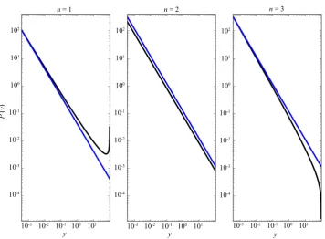
We observe an exact power-law distribution P y

( )

 y−1 with power-law exponent −1 in n=2 dimensions. Figure 1 shows the randomly sampled densities y in n=1, 2, 3 dimensions.

3.2. Exponentials

In this section, radially symmetric exponential shapes as given by (1.3) in n=1, 2, 3 dimensions are analyzed. The exponential defines a continuous, bijective mapping y: 0,

[ ]

R →_Aexp

(

−λR

)

,A_. The inverse is given by

( )

1

log y x y A λ   = − _{ }   and the derivative of the inverse by

( )

1

d 1

. dyx y λ y

−

= −

In n dimensions, random variable transformation (1.1) yields the densities P y

( )

:

( )

1 1 2 2 2 1 3 3 1 1 2 log 2 3 3. log y n R y

P y y n

(4)

[image:4.595.137.494.80.342.2]

Figure 1. Radially uniform random sampling of Gaussian functions in n = 1, 2, 3 dimensions yield exact and approximate power-law distributions (black curves). In the case n = 1, an exact power-law with exponent −1 is obtained. The blue curves are the Padé approximants to the exact distrubutions

P(y). For visualization purposes, the blue curves are offset by a fixed amount.

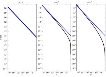
In the exponential case, an exact power-law distribution P y

( )

with exponent −1 is obtained in one dimension (in n = 1). In n=2, 3 dimensions, the distributions P y

( )

approximately follow a power-law for

0

y→ . This behaviour is visualized in Figure 2 and analyzed quantitatively using Padé approximants further below.Figure 2 shows the randomly sampled densities P y

( )

in n dimensions.

3.3. Power-Laws

Finally, we ask which amplitude distribution P y

( )

is obtained by randomly sampling functions that already follow a power-law. The function y x

( )

in arbitrary dimensions is given by (1.4). In order to obtain a continuous, bijective mapping, domain and co-domain are set accordingly, y:

[ ]

ε,R → AR−α,Aε−α_, where

0<ε 1. The inverse is given by

( )

1 1

x y y

A

α

−

=

and the derivative of the inverse by

( )

1 1

d 1

.

dyx y A y

α

− −

= −

Random variable transformation in n=1, 2, 3 dimensions yields the three densities

( )

1 1

2 1

2 2

3 1

3 3

1

2

3

3.

y n

AR

P y y n

A R

y n

A R

α

− −



= 

 

=_ =

 

= 

(5)

[image:5.595.136.495.81.341.2]

Figure 2. Random sampling of exponential functions in n = 1, 2, 3 dimensions yield an exact power-law distribution with exponent −1 for n = 1. For n = 2, 3, an approximate power-law be- ha- viour is observed for y→0. Blue curves are the Padé approximants to the exact distrubutions P(y). For visualization purposes, the blue curves are offset by a fixed amount.

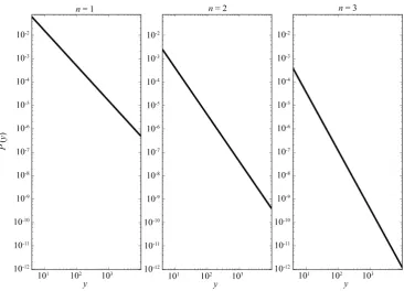
In this case, exact power-laws with exponents n 1

α

− − are obtained in any dimension n=1, 2, 3. Figure 3

shows the randomly sampled densities P y

( )

.

4 .

Padé

Approximants

In Figure 1 and Figure 4, an approximate power-law behaviour of P y

( )

is observed for small values of y. In order to quantify this behaviour, we computed Padé approximants of order

( )

1,1 of the densities P y

( )

[11]. The approximants were calculated from the Taylor expansions of P y

( )

at the left border of the codomain of y x

( )

. For first order approximations, the densities P y

( )

can be approximated by functions of

the form a

by+c. As derived above, sampling a Gaussian in two dimensions or an exponential in one

dimension, exact power-laws with exponent −1 are obtained. In these cases, the Padé approximants yield the exact result. In the other cases, the Padé approximants yield functions that follow the density P y

( )

close to the origin. The Padé coefficients are given in Table 1.

5. A Numerical Example

A small numerical example is presented to illustrate the connection between the theoretically derived results and possible implications for experimental data. Consider an experiment where Gaussian shaped signals occur at a random distance x to a fixed sensor. This situation is illustrated in the left panel of Figure 3, with the sensor

( )

S at the center. In analogy to the analytical derivations, all events are assumed to occur within a two-dimensional disc of radius R. The amplitude y of the event measured at site S depends on the random distance

(6)

Figure 3. Random sampling of power-law functions in n dimensions produces exact power-law distributions P(y) with exponent n 1

α

− − .

Figure 4. Numerical example. In the left panel, a generic experimental setting is illustrated. A sensor (S) is placed at a fixed location and Gaussian shaped events occur at random distances x from the sensor S, within a disc shaped 2D region of radius R. The amplitude of the Gaussian y measured at the sensor site decreases with increasing distance x. The right panel shows the empirical distribution of event amplitudes P(y) (blue circles, n = 104 samples) in double logarithmic coordinate axes to emphasize the exact power-law character of the empirical distribution. A power-law fit to the data (black solid line) yields an exponent of ˆα = −0.985, a close fit to the theoretically derived exponent α = −1.

in the right panel of Figure 4), a result close to the theoretically derived distribution P y

( )

∝y−α with exponent α = −1.

6. Discussion

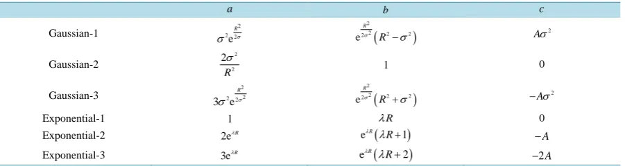
[image:6.595.131.498.82.346.2]

(7)

[image:7.595.91.542.127.247.2]

Table 1. First-order Padé approximants of the densities P(y) are given by a

by+c. The table shows the coefficients for

Gaussian and exponential functions in n dimensions, denoted Gaussian-n and Exponential-n.

a b c

Gaussian-1 2_e22

R σ

σ

(

)

2

2 2 2

2

e

R R

σ ₋_σ Aσ2

Gaussian-2

2 2

2

R

σ

1 0

Gaussian-3

2 2 2 2

3 e

R σ

σ

(

)

2

2 2 2

2

e

R R

σ ₊σ −Aσ2

Exponential-1 1 λR 0

Exponential-2 2eλR _eλR(λ +_R ₁)

A

−

Exponential-3 3eλR _eλR(_{λ +}_R ₂)

2A

−

based upon a realistic scenario in experimental sciences. A signal of a given shape, e.g. a Gaussian or an exponential, is measured by a sensor at a random distance x to the signal maximum. Random sampling arises when the Gaussian or exponentially shaped signal occurs randomly distributed across space (with density P x

( )

) and the sensor resides at a fixed site. Our derivation shows that two-dimensional Gaussians and one-dimensional exponentials lead to exact power-law densities with exponent −1 and that approximate power-law densities arise in other dimensions. Indeed, this mechanism has been observed experimentally in dynamic fluorescence microscopy of subcellular calcium currents [12]. The result is of interest as it provides a simple and realistic mechanism that produces exact power-laws. Power-laws are often associated with specialized mechanisms such as phase transitions in complex systems, bifurcation points of dynamical systems or systems displaying self- organized criticality and relatively few authors have considered alternative mechanisms [6]. The mechnism presented here is generic and may serve as an alternative hypothesis in cases where power-law distributions are observed in experimental settings.

References

[1] Hohenberg, P.C. and Halperin, B.I. (1977) Theory of Dynamic Critical Phenomena. Reviews of Modern Physics, 49, 435-479. http://dx.doi.org/10.1103/RevModPhys.49.435

[2] Mitzenmacher, M. (2003) A Brief History of Generative Models for Power Law and Lognormal Distributions. Internet Mathematics, 1, 226-251. http://dx.doi.org/10.1080/15427951.2004.10129088

[3] Montroll, M. and Shlesinger, M.F. (1983) Maximum Entropy Formalism, Fractals, Scaling Phenomena, and 1/f Noise: A Tale of Tails. The Journal of Chemical Physics, 32, 209-230. http://dx.doi.org/10.1007/BF01012708

[4] Newman, M.E.J. (2005) Power Laws, Pareto Distributions and Zipfs Law, Contemporary Physics.

http://dx.doi.org/10.1080/00107510500052444

[5] Stanley, H.E. (1999) Scaling, Universality, and Renormalization: Three Pillars of Modern Critical Phenomena. Re-views of Modern Physics, 71, S358-S366. http://dx.doi.org/10.1103/RevModPhys.71.S358

[6] Sornette, D. (2004) Critical Phenomena in Natural Sciences: Chaos, Fractals, Selforganization, and Disorder: Concepts and Tools. Springer, New York.

[7] Malmgren, R.D., Stouffer, D.B., Motter, A.E. and Amaral, L.A.N. (2008) A Poissonian Explanation for Heavy Tails in E-Mail Communication. Proceedings of National Academy Science of USA, 105, 18153-18158.

http://dx.doi.org/10.1073/pnas.0800332105

[8] Sornette, D. (1998) Multiplicative Processes and Power Laws. Physical Review E, 57, 4811-4813.

http://dx.doi.org/10.1103/PhysRevE.57.4811

[9] Touboul, J. and Destexhe, A. (2010) Can Power-Law Scaling and Neuronal Avalanches Arise from Stochastic Dy-namics? PLoS One, 5, e8982.

[10] Ramachandran, K.M. and Tsokos, C.P. (2009) Mathematical Statistics with Applications. Academic Press. [11] Jr. Baker, G.A. and Graves-Morris, P. (1996) Padé Approximants. Cambridge University Press, New York.

[12] Ríos, E., Shirokova, N., Kirsch, W.G., Pizarro, G., Stern, M.D., Cheng, H. and González, A. (2001) A Preferred Am-plitude of Calcium Sparks in Skeletal Muscle. Biophysical Journal, 80, 169-183.

(8)

currently publishing more than 200 open access, online, peer-reviewed journals covering a wide range of academic disciplines. SCIRP serves the worldwide academic communities and contributes to the progress and application of science with its publication.

Other selected journals from SCIRP are listed as below. Submit your manuscript to us via either