Numerical Study on Steady Magnetohydrodynamics
(MHD) Flow and Heat Transfer in a Heated Rectangular
Electrically Insulated Duct under the Action of Strong
Oblique Transverse Magnetic Field
Muhim Chutia
Department of Mathematics Mariani College, Mariani-785634
P. N. Deka
Department of Mathematics Dibrugarh University, Dibrugarh-786004
ABSTRACT
Steady laminar magnetohydrodynamics flow and heat transfer of an electrically conducting fluid in a rectangular duct in the presence of oblique transverse magnetic field is considered. The walls of the duct are electrically insulated and kept at constant temperature( ). The fluid is kept in motion by a constant pressure gradient and the viscous and Joule dissipations are considered in the energy equation. The dimensionless coupled partial differential equations are solved numerically employing finite difference method for velocity, induced magnetic field and temperature distribution. The computed results for velocity, induced magnetic field and temperature are visualized in terms of graphics for different values of oblique angle( ), Hartmaan number , Prandtl number and the aspect ratio , the ratio of the length to the breadth.
Keywords
MHD flow, electrically insulated walls, rectangular duct, heat transfer, finite difference method, aspect ratio.
1. INTRODUCTION
The MHD flow of an electrically conducting fluid in a channel of duct has received great attention due to its applications in MHD power generators, pumps, nuclear fusion reactors, energy storage etc. The basic set of equations which describe MHD flow and heat transfer are the combination of the Navier-Stokes equations of fluid mechanics, Maxwell’s equations of electromagnetism and energy equation of thermodynamics. Hartmaan and Lazarus, 1937 [1] first studied the influence of transverse uniform magnetic field on the flow of an electrically conducting viscous incompressible fluid between two infinite parallel insulating plates. Umavathi et.al.[2] studied numerically the steady natural convection flow in a vertical rectangular duct with isothermal wall boundary conditions for non-magnetic case. Umavathi et. al. [3] also investigated the MHD free convection flow in a vertical rectangular duct for laminar and fully developed regime taking into consideration the effect of Ohmic heating and viscous dissipation numerically using finite difference method of second order accuracy. Garner et. al. [4] had acquired some results for MFD flow of circular pipe in a transverse magnetic field with heat transfer experimentally. Morley et. al. [5] studied fully developed, gravity-driven flow in an open channel of arbitrary electrical conductance and orientation to an applied magnetic field numerically. Al-Khawaja et al. [6] studied numerically the Magneto-Fluid-Mechanics flow in a circular pipe with heat transfer and for the case of uniform wall heat flux with forced convection. Al-Khawaja et al. [7] also obtained the solution for MFD flow of square duct using spectral method for the case of uniform wall temperature. Ibrahim [8] studied numerically MHD flow
equations in a rectangular duct in the presence of transverse external oblique magnetic field for values of Hartmann number . He employed Chebyshev collocation method to solve partial differential equations. Hosseinzadeh et.al.[9] carried out a numerical study using boundary element method(BEMs) for steady MHD flow having arbitrary wall conductivity. Recently, Sarma et. al.[10] have investigated numerically steady MHD flow of liquid metal through a square duct under the action of strong transverse magnetic field. They have considered the wall of the duct are electrically insulated as well as isothermal.
In this present work, the problem investigated is the steady laminar MHD flow of an electrically conducting viscous incompressible fluid through a rectangular duct with heat transfer under the action of oblique transverse magnetic field. The fluid is kept in motion by a constant pressure gradient and viscous and Joule dissipation are considered in the energy equation. The walls of the duct are kept at constant temperature( ) and electrically insulated. The coupled equations of the momentum(motion), energy and magnetic induction equation are solved numerically using finite difference approximations to obtain the velocity, temperature and induced magnetic fields. The results for velocity, induced magnetic field and temperature are visualized in terms of graphics for different values of the flow parameters.
2.
FORMULATION OF THE PROBLEM
The steady laminar two dimensional motion of an electrically conducting fluid in a rectangular duct in the presence of oblique transverse magnetic field is considered. The length and breadth of the rectangular cross section of the duct are and . It is assumed that all the plates of the duct are maintained at constant temperature and electrically insulated. Two parallel walls of the duct are at and at
and other parallel walls of the duct are at and at
. A constant pressure gradient is applied in the -direction, which supports the flow and the direction of the flow. The applied uniform magnetic field acts in a direction lying in the plane but makes an angle with the -axis, which induces a magnetic field in the flow direction and and are the resolved part of . In this
investigation, we consider the following assumptions:
(i) The flow is laminar, steady and fully developed. (ii) The fluid is finitely conducting.
(iii) In the energy equation, we have considered viscous dissipation and Joule heating.
Fig.1 Physical configuration of rectangular duct flow
Under above assumptions, the velocity and magnetic field will be the following form
Where .
3. GOVERNING EQUATIONS
The governing equations of MHD flow with energy equation are:-
(1)
(2)
(3)
(4)
(5)
(6)
(7)
Where is the current density due to the magnetic field, is the viscous dissipation function, is the electric field intensity, is the temperature, ρ is density of the fluid, σ is the electrical conductivity, , is the co-efficient of viscosity, is the kinematic viscosity, is magnetic permeability and is the magnetic diffusivity. Using (1) and (2) in equation (4), we get (8)
In steady case, and using velocity and magnetic field distribution stated as above, equations (3), (5) and (8) become (9)
2 =0 (10)
(11)
The corresponding boundary conditions are as follows: (12) The above equations (9), (10) and (11) can be transformed into dimensionless form using the following dimensionless quantities as , , , , (13)
Where, , is the aspect ratio of the duct. Using dimensionless quantities (10) in equations (9), (10) and (11) and dropping asterisks, we obtain (14)
(15)
(16)
Where, , is the Hartmaan number
, is the Prandtl number
, is the magnetic Reynolds number
(17)
The dimensionless coupled linear partial differential equations (14), (15) and (16) associated with the boundary conditions (17) are solved numerically using finite difference scheme and Matlab programming. In this numerical technique we have descrretized governing equations (14), (15) and (16) along with the boundary conditions (17). Computational domain is divided into a uniform grid system. We have descretized both the second derivative and first derivative which appearing in the governing equations using the central difference of second order accuracy followed by Schmidit[11]. Therefore the resultant difference equations for equations (14), (15) and (16) are as follows
(18)
(19)
(20)
Where, ,
, , ,
,
, , ,
, ,
are constants and and .
The corresponding descretized boundary conditions are
(21)
Where refers to and refers to , and denote the number of grids inside the computational domain in the direction of and respectively. The values ,
and in the equations (18), (19) and (20) with the
parameters , , and have been iterated using boundary conditions (21). We repeat the process, till the converged solution for , and in the grid system
are obtained.
4. RESULT AND DISCUSSIONS
Inthis study a numerical investigation on MHD flow and heat transfer in a rectangular duct under the action of strong oblique transverse magnetic field is considered. Strong imposed magnetic field creates a Lorentz force , which retards the flow and produces a pressure drop in addition to viscous pressure drop. So we have considered electrically insulating walls to reduce the pressure drop phenomena in the duct.
The basic coupled linear partial differential equations are solved using finite difference method. Numerical investigations are carried out in the spatial domain and using Matlab. During numerical computation, we have considered , so that the stability condition is fulfilled. It is observed that the Prandtl number
gives no effect to the velocity and induced magnetic field, as can be seen from Eqn. (14) and (16). The results are drawn and shown graphically for the fixed aspect ratio and different values of parameters inclination angle( ), Hartmaan number , Prandtl number and aspect ratio on velocity , temperature and induced magnetic field.
If we consider , then applied magnetic field is parallel to -axis and orthogonal to the -axis. The walls normal to the applied magnetic field are called Hartmaan walls and the boundary layers adjacent to these walls are called Hartmaan layers. In Hartmaan layers, the velocity profile is basically determined from the balance between Lorentz and viscous forces, and the thickness of these layers scales as , where is the Hartmaan number. The walls parallel to the magnetic field direction are called side walls, and boundary layers adjacent to these walls are called side walls, whose thickness scales as . The thickness of side layers are larger than Hartmaan layers.
Fig.2 Induced magnetic field at , ,
, and .
x/a
y
/A
a
0 0.1 0.2 0.3 0.4 0.5 0.6 0.7 0.8 0.9 1 0
0.1 0.2 0.3 0.4 0.5 0.6 0.7 0.8 0.9 1
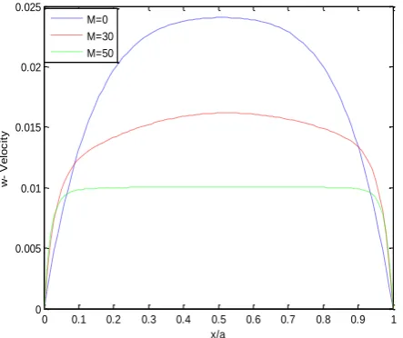
Fig.3 Velocity distribution along - axis at various for , , and
[image:4.595.62.284.84.270.2]In figures from 2 to 8, we have shown the velocity, induced magnetic field and temperature at fixed value of .
Fig.4 Velocity distribution along - axis at various for , , and .
Figure 2 is plotted for induced magnetic field, which are lines of current density at and , keeping other parameters constant, the induced magnetic field is symmetric with respect to - axis for Figure 2 establishes the results of [8]. Figures 3 and 4 show the velocity profiles along Hartmaan and side walls respectively, from these
Fig.5 Temperature along - axis at various for
, , and .
figures, we have noticed that velocity profile along Hartmaan layers become more flatten than side layers due to increasing values of , i.e. Hartmaan layers are thinner than side layers.
Fig.6 Temperature along - axis at various for
, , and .
The influence of flow parameters on temperature are shown in figures from 5 to 8. In figures 5 and 6 temperature distribution are visualized at various Hartmann numbers along and -axes respectively. We have observed that temperature distribution increases in both axes as Hartmaan number
0 0.1 0.2 0.3 0.4 0.5 0.6 0.7 0.8 0.9 1 0
0.005 0.01 0.015 0.02 0.025
x/a
w
-
V
e
lo
c
it
y
M=0 M=30 M=50
0 0.1 0.2 0.3 0.4 0.5 0.6 0.7 0.8 0.9 1
0 0.005 0.01 0.015 0.02 0.025
y/Aa
w
-V
e
lo
c
it
y
M=0 M=30 M=50
0 0.1 0.2 0.3 0.4 0.5 0.6 0.7 0.8 0.9 1 0
1 2 3 4 5 6 7 8 9x 10
-3
T
-T
e
m
p
e
ra
tu
re
y/Aa
M=30 M=40 M=50
0 0.1 0.2 0.3 0.4 0.5 0.6 0.7 0.8 0.9 1
0 0.005 0.01 0.015 0.02 0.025 0.03
x/a
T
(T
e
m
p
e
ra
tu
re
)
[image:4.595.322.538.374.572.2]Fig.7 Temperature along - axis at various for
[image:5.595.323.543.96.303.2], , and .
Fig.8 Temperature along - axis at various for
, , and .
increases, along -axis temperature distributions are parabolic in nature, but along -axis its profiles are shape. Figures 7 and 8 are plotted for temperature at various along and -axes respectively, it is noticed that temperature increases along both axes with the increasing values of .
[image:5.595.64.286.343.546.2]
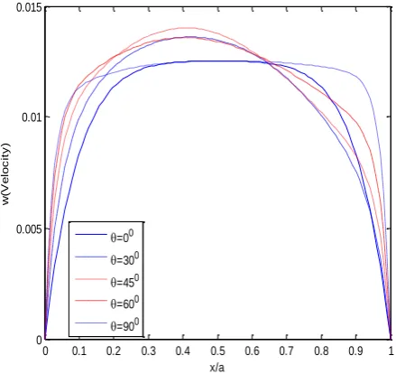
Fig.9 Velocity distribution along - axis at various for , , and .
Fig.10 Temperature along - axis at various for
, , and .
Figure 9 presents the effect of on velocity , it can be seen that the velocity increases from to , then decreases from to . It establishes the result of [9]. Figure 10
0 0.1 0.2 0.3 0.4 0.5 0.6 0.7 0.8 0.9 1
0 0.002 0.004 0.006 0.008 0.01 0.012 0.014 0.016 0.018 0.02
y/Aa
T
(T
e
m
p
e
ra
tu
re
)
Pr=0.71 Pr=1.00 Pr=1.50
0 0.1 0.2 0.3 0.4 0.5 0.6 0.7 0.8 0.9 1
0 0.01 0.02 0.03 0.04 0.05 0.06
x/a
T
(T
e
m
p
e
ra
tu
re
)
Pr=0.71 Pr=1.00 Pr=1.50
0 0.1 0.2 0.3 0.4 0.5 0.6 0.7 0.8 0.9 1
0 0.005 0.01 0.015
x/a
w
(V
e
lo
c
it
y
)
=00 =300 =450 =600 =900
0 0.1 0.2 0.3 0.4 0.5 0.6 0.7 0.8 0.9 1
0 0.005 0.01 0.015 0.02 0.025 0.03
x/a
T
(T
e
m
p
e
ra
tu
re
)
[image:5.595.321.541.362.574.2]shows temperature at various for , ,
Fig.11 Induced magnetic field at for ,
, and .
and . Temperature is found to increase as increases and the temperature gradient is greater at the Hartmaan layers than in core region of the duct.
Fig.12 Induced magnetic field at for ,
, and .
In figures from 11 to 14, we have plotted the current density lines for at , , ,
. In figure 11, we have noticed that the induced
magnetic field (lines of current density) is symmetric with
Fig.13 Induced magnetic field at for ,
, and .
respect to -axis for . It can be seen that the boundary layers are concentrated near boundary walls along parallel to both and -axes for . Figure 12 presents the induced
Fig.14 Induced magnetic field at ,
, and .
magnetic field for , it is symmetric with respect to the line . Moreover it can be seen that the boundary layers are concentrated near the corners in the direction of the oblique magnetic field. But it is anti-symmetric with respect
x/a
y
/A
a
0 0.1 0.2 0.3 0.4 0.5 0.6 0.7 0.8 0.9 1
0 0.1 0.2 0.3 0.4 0.5 0.6 0.7 0.8 0.9 1
M=100 A=1
x/a
y
/A
a
0 0.1 0.2 0.3 0.4 0.5 0.6 0.7 0.8 0.9 1
0 0.1 0.2 0.3 0.4 0.5 0.6 0.7 0.8 0.9 1
M=100 A=1
x/a
y
/A
a
0 0.1 0.2 0.3 0.4 0.5 0.6 0.7 0.8 0.9 1
0 0.1 0.2 0.3 0.4 0.5 0.6 0.7 0.8 0.9 1
M=100 A=1
x/a
y
/A
a
0 0.1 0.2 0.3 0.4 0.5 0.6 0.7 0.8 0.9 1
0 0.1 0.2 0.3 0.4 0.5 0.6 0.7 0.8 0.9 1
Fig.15 Velocity distribution along - axis at various for , , and .
to the -axis and line for and respectively.
The influence of aspect ratio on velocity and temperature distribution are drawn in figures 15 and 16 respectively. Induced magnetic fields are presented for different values of in figures 17, 18 and 19. It can be seen that the velocity,
Fig.16 Temperature distribution along - axis at various for , , and .
Fig.17 Induced magnetic field at for ,
, and .
temperature and induced magnetic field increase as increases and they are looked more flat for large value of . The effect flow parameters on velocity, magnetic field and temperature showing in terms graphics are well known characteristic of MHD flow with heat transfer in duct.
This paper establishes the characteristic features of MHD duct flow. The effect of variation of aspect ratio, heat transfer effect, wall conductivity, strength of applied magnetic field and direction of applied magnetic field are studied numerically. Desired accuracy may be achieved with more appropriate meshing. Wall conductance ratio may be considered in such problems, which may considerably change the results in MHD duct flow for very high Hartmaan number. In such situation extra complexities may appear in the dynamics and more appropriate algorithm may be required to obtain the solution.
Fig.18 Induced magnetic field at for ,
, and .
0 0.5 1 1.5
0 0.002 0.004 0.006 0.008 0.01 0.012 0.014
x/a
w
(V
e
lo
c
it
y
)
A=0.5 A=1.0 A=1.5
0 0.2 0.4 0.6 0.8 1 1.2 1.4 1.6 1.8 2
0 0.005 0.01 0.015 0.02 0.025 0.03 0.035
x/a
T
(T
e
m
p
e
ra
tu
re
)
A=1.0 A=1.5 A=2.0
x/a
y
/A
a
0 0.1 0.2 0.3 0.4 0.5 0.6 0.7 0.8 0.9 1
0 0.1 0.2 0.3 0.4 0.5 0.6 0.7 0.8 0.9 1
A=1.0
x/a
y
/A
a
0 0.5 1 1.5
0 0.1 0.2 0.3 0.4 0.5 0.6 0.7 0.8 0.9 1
Fig.19 Induced magnetic field at for ,
, and .
Further, we can extend this research work to include the buoyancy force by considering the duct aligned to the vertical direction. In such cases a dimensionless independent parameter Grashof number will appear in the governing equations besides Hartmaan number , oblique angle , Prandtl number and aspect ratio . This will create an extra complexity to the problem.
5. REFERENCES
[1] Hartmaan J., Lazarus F. 1937. Experimental investigations on the flow of mercury in a homogeneous magnetic field, K. Dan. Vidensk. Selsk. Mat. Fys. Meed. Vol. 15, pp. 1-45.
[2] Umavathi J. C., Chamka A. J. 2013 Steady natural convection flow in a vertical rectangular duct with isothermal wall boundary conditions, International Journal of Energy and Technology, 5(20), pp. 1-10.
[3] Umavathi J. C., Liu I. C., Kumar J. P., Pop I. 2011. Fully developed magneto convection flow in a vertical rectangular duct, Heat and Mass Transfer: 47(1)., pp. 1-11.
[4] Garner R. A., Lykouidis P.S. 1971. Magneto-Fluid-Mechanics Pipe Flow in a Transverse Magnetic Field
Part Two. Heat Transfer. J. Fluid Mech., Vol. 48 Part 1, pp. 129-141.
[5] Morley N. B., Abdou M. A. 1997. Study of fully developed, liquid-metal, open-channel flow in a nearly coplanar magnetic field, Fusion Technology, Vol. 31, pp. 135-153.
[6] Al-Khawaja M. J., Gardner R. A., Agarwal R. 1994. Numercal study of Magneto-Fluid-Mechanics forced convection pipe flow. Engineering Journal of Qatar University, Vol. 7, pp. 115-134.
[7] Al-Khawaja M. J., Mohammed J., Selmi, Mohamed. 2006. Highly Accurate Solution of a Laminar Square Duct in a Transverse magnetic Field With Heat Transfer Using Spectral Method. Journal of Heat Transfer, Vol. 128, pp. 413-417.
[8] Ibrahim C. 2011. Solution of magnetohydrodynamic flow in a rectangular duct by Chebyshev collocation Method, International Journal for Numerical Method in Fluids, Vol. 66, pp. 1325-1340.
[9] Hosseinzadeha H., Dehghana M., D. Mirzaeib D. 2012. The boundary elements method for magnetohydrodynamics(MHD) channel flows at high Hartmaan numbers, AMS classification: 65N38.
[10]D. Sarma, G. C. Hazarika and P. N. Deka, 2013. Numerical study of liquid metal MHD flow through a square duct under the action of strong transverse magnetic field, International Journal Computer Applications(0975-8887),Vol.-71,No.8.
[11]Jain M. K., Iyenger S. R. K., Jain R.K. 1994. Computational Method for Partial Differential Equations, Wiley Eastern Limited.
[12] Sutton G. W., Sherman A. 1965. Engineering Magnetohydrodynamics, Dover Publication, Inc. Mineola, New York.
[13]Cramer K. R., Pai Shih-I. 1973. Magnetofluid Dynamics for Engineers and Applied Physicists, Scripta Publishing Company, Washington, D. C.
[14] Muller U., Buhler L. 2001. Magnetohydrodynamics in Channels and containers, Springer.
[15]Leite E. P. 2010. Matlab-Modelling, Programming and Simulations, Sciyo.
[16]Mathews J. H., Fink K. D. 2009. Numerical Methods using Matlab, PHI Learning Private Limited.
x/a
y
/A
a
0 0.2 0.4 0.6 0.8 1 1.2 1.4 1.6 1.8 2
0 0.1 0.2 0.3 0.4 0.5 0.6 0.7 0.8 0.9 1