Experimental Design for Optimizing a Mixture of Materials plus an Evaporating Solvent

http://dx.doi.org/10.4236/am.2015.610154

How to cite this paper: Fernandi, M., Decastri, D., Bazzurri, M. and Clementi, S. (2015) Experimental Design for Optimizing a Mixture of Materials plus an Evaporating Solvent. Applied Mathematics, 6, 1740-1746.

http://dx.doi.org/10.4236/am.2015.610154

Experimental Design for Optimizing

a Mixture of Materials plus an

Evaporating Solvent

Mauro Fernandi

, Diego Decastri

, Matteo Bazzurri

, Sergio Clementi

1_{Flint Group, Cinisello Balsamo, Milano, Italy}

2_{Chemistry Department, University of Perugia, Perugia, Italy} 3_{M.I.A. Multivariate Infometric Analysis Srl, Perugia, Italy}

Email: *_{[email protected]}

Received 10 August 2015; accepted 15 September 2015; published 18 September 2015

Copyright © 2015 by authors and Scientific Research Publishing Inc.

This work is licensed under the Creative Commons Attribution International License (CC BY). http://creativecommons.org/licenses/by/4.0/

Abstract

The paper illustrates a further new way of using the CARSO procedure for response surfaces analyses derived from experimental designs based on Double Circulant Matrices (DCMs). We re-port a case study regarding a design based on a mixture of three chemicals plus an evaporating solvent, in order to compare the relative reliability of designs based either on 3 only or on all 4 factors. We show that both designs give the same results, but the second is preferable because it represents the real situation at the beginning of the process, so that it is possible to know the re-quired amount of solvent that should be used for each experiment. Obviously this applies to any number of factors using the correspondent DCM.

Keywords

CARSO Procedure, Design Strategies, Circulant Matrices (DCM), Optimization

1. Introduction

Following our previous paper published last November [1], where we have showed a new strategy for collecting the data needed for defining a response surface on the basis of an innovative strategy that requires only a very low number of experimental data, based on Double Circulant Matrices (DCMs), thus obtaining better results with respect to the previous method based on D-optimal design [2], for the objective of industrial research in reaching the best level of technological properties the mixture is expected to exhibit. The DCMs have similar

requirements to Central Composite Designs (CCDs), which represent the best way to generate response surfaces. The final response surface model is obtained by the formerly developed CARSO method [3], where the surface equation is derived by a PLS model on the expanded matrix, containing linear, squared and bifactorial terms, and studied at extreme points by Lagrange analysis.

Now we present the results for the cases where one of the components of the mixture is a solvent, which va-porizes during the deposition. Indeed this situation is quite frequent in painting industrial materials and we wish to understand what may be the best way in deciding the experimental design. The most intriguing case is a mix-ture of three materials and an evaporating solvent.

2. Problem Formulation

In principle it would be possible using either a three or a four materials mixture, depending upon excluding or including the solvent, but this would generate two different nomenclatures for the same formula, which may be difficult to handle. Therefore we decided that, since the solvent must be used from the beginning, it seems ap-propriate to include it into the experimental design, even if at the end of the process it will not be present any more. This will simplify a lot the handling of the experimental work. The solvent is a temporary ingredient which brings the solid chemicals into a fluid state. It is however desirable that the mixture should very quickly assume the solid state. Solvents remain in the mixture during the whole process of printing until they are re-moved immediately after impression. They are practically absent in the finished print, but provide an extremely important expedient in all stages before drying. The objective of this paper is to investigate whether the experi-mental designs with 3 or 4 variables give the same or different results.

3. Experimental Design and Data Collection

The experimental design with coded data is that used in ref. 1 on DCM4, but using only one central point (Table 1), whereas in Table 2 we show the decoded (true) values of the variables, and inTable 3 we report the true compositions of our nine mixtures (objects).

Table 1. Coded values of 4 variables in a DCM4 (see Ref. [1]).

x1 x2 x3 x4

e11 −1 −0.58 0.58 1

e12 −0.58 0.58 1 −1

e13 0.58 1 −1 −0.58

e14 1 −1 −0.58 0.58

e31 −1 0.58 1 −0.58

e32 0.58 1 −0.58 −1

e33 1 −0.58 −1 0.58

e34 −0.58 −1 0.58 1

cc 0 0 0 0

Table 2. Real values of 4 variables by simple linear functions, on defining the highest and lowest levels for each variable by the equation in the last row.

Level x1 x2 x3 x4

−1 4.40 1.10 50.00 8.00

−0.58 5.03 1.27 62.60 8.42

0.58 6.77 1.73 97.40 9.58

1 7.40 1.90 110.00 10.00

0 5.90 1.50 80.00 9.00

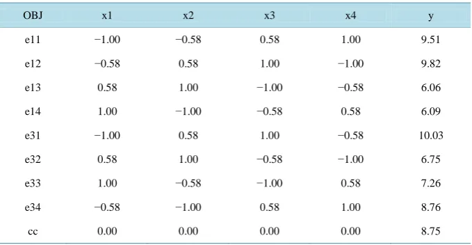
The experimental collection of the technological property on polypropylene for each of these mixtures is re-ported in Table 4. The variables x1, x2 and x3 are solid components, while x4 is the volatile part of the mixture.

As we stated in our previous paper [1] the response property should be modelled by the linear, quadratic and bifactorial terms: in other terms the matrix expansion is needed for obtaining a quadratic model.

x1 x2 x3 x4 x12 _x22 _x32 _x42 _{x1x2 x1x3 x1x4 x2x3 x2x4 x3x4}

On using only the non evaporating compounds the expansion is the following:

x1 x2 x3 x12 x22 x32 x1x2 x1x3 x2x3

After expansion the X block is reported in the following Table 5.

4. Linear PLS Models on an Expanded Matrix

For maintaining the maximum of the symmetry of the experimental design we decided to use a single point at the centre. The absence of replicates does not destroy the extraction of systematic information, if it exists in the experimental plan.

Table 3. Real values of the compositions of the nine mixtures (objects) on reporting the real values of Table 2 instead of the coded ones in Table 1.

x1 x2 x3 x4

e11 4.40 1.34 92.00 10.00

e12 5.30 1.66 110.00 8.00

e13 6.50 1.90 50.00 8.60

e14 7.40 1.10 68.00 9.40

e31 4.40 1.66 110.00 8.60

e32 6.50 1.90 68.00 8.00

e33 7.40 1.34 50.00 9.40

e34 5.30 1.10 92.00 10.00

cc 5.90 1.50 80.00 9.00

Table 4. Experimental responses of the coded compositions of the nine mixtures

OBJ x1 x2 x3 x4 y

e11 −1.00 −0.58 0.58 1.00 9.51

e12 −0.58 0.58 1.00 −1.00 9.82

e13 0.58 1.00 −1.00 −0.58 6.06

e14 1.00 −1.00 −0.58 0.58 6.09

e31 −1.00 0.58 1.00 −0.58 10.03

e32 0.58 1.00 −0.58 −1.00 6.75

e33 1.00 −0.58 −1.00 0.58 7.26

e34 −0.58 −1.00 0.58 1.00 8.76

We first adopted linear models on an expanded matrix for our need to develop, within the CARSO method [3], the GOLPE procedure [4] [5], aimed to describe the y parameter by a quadratic model, in order to find out the best combination of x variables for its highest value. Indeed, for searching a minimum we should find the maximum of the inverse of y.

The characteristics of the models DCM4 and DCM4-S are very close. Both use nine objects, one dimension, show good plots, and similar values (0.33 and 0.35) for the SDEC (Standard Deviation of Error of Computations) and for the y variance explained (93.6% and 93.1%). However, the best comparison can be derived by the coef-ficients evaluating the relative importance of each x parameter (GAM1) listed inTable 6.

Comparative Evaluation of Variables Contributions

The most important step of the SIMCA philosophy is the dissection of each element of a table of data into two contributions, relative to the objects (scores, that evaluate the relative position of each of them into the reduced

Table 5. Coded values of DCM and DCM4-S.

DCM4-S x1 x2 x3 x12 _x22 _x32 _{x1x2 x1x3 x2x3}

1 2 3 4 5 6 7 8 9 10 11 12 13 14

DCM4 x1 x2 x3 x4 x12 _x22 _x32 _x42 _{x1x2 x1x3 x1x4 x2x3 x2x4 x3x4}

e11 −1 −0.58 0.58 1 1.00 0.34 0.34 1.00 0.58 −0.58 −1.00 −0.34 −0.58 0.58

e12 −0.58 0.58 1 −1 0.34 0.34 1.00 1.00 −0.34 −0.58 0.58 0.58 −0.58 −1.00

e13 0.58 1 −1 −0.58 0.34 1.00 1.00 0.34 0.58 −0.58 −0.34 −1.00 −0.58 0.58

e14 1 −1 −0.58 0.58 1.00 1.00 0.34 0.34 −1.00 −0.58 0.58 0.58 −0.58 −0.34

e31 −1 0.58 1 −0.58 1.00 0.34 1.00 0.34 −0.58 −1.00 0.58 0.58 −0.34 −0.58

e32 0.58 1 −0.58 −1 0.34 1.00 0.34 1.00 0.58 −0.34 −0.58 −0.58 −1.00 0.58

e33 1 −0.58 −1 0.58 1.00 0.34 1.00 0.34 −0.58 −1.00 0.58 0.58 −0.34 −0.58

e34 −0.58 −1 0.58 1 0.34 1.00 0.34 1.00 0.58 −0.34 −0.58 −0.58 −1.00 0.58

cc 0 0 0 0 0.00 0.00 0.00 0.00 0.00 0.00 0.00 0.00 0.00 0.00

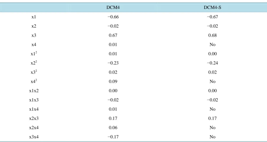
Table 6. Comparison of the parameters gamma 1 for the two models.

DCM4 DCM4-S

x1 −0.66 −0.67

x2 −0.02 −0.02

x3 0.67 0.68

x4 0.01 No

x12 _{0.01 0.00}

x22 _{−0.23 −0.24}

x32 _{0.02 0.02}

x42 0.09 No

x1x2 0.00 0.00

x1x3 −0.02 −0.02

x1x4 0.01 No

x2x3 0.17 0.17

x2x4 0.06 No

space of the main information) and to the variables (loadings, that evaluate the relative importance of each vari-able so that the sum of their squares is equal to one) [6].

In PCA, where there are no dependent variables, the parameters of x variables are called beta and their sum of squares is equal to one. The same parameters in PLS are called gamma: they are very similar to the beta, but their sum of squares is not equal to one. However, the program inventors say that using gamma instead of beta gives better predictions [7].

The terms gamma 1 reported in Table 6 indicate the gamma values (i.e. the relative importance of each vari-able) for the first latent variable. The results obtained are the core of this paper. The first and main result is the almost identical gammas for the two models, thus demonstrating that the experimental designs with four vari-ables (including the solvent) and that with 3 varivari-ables (without the solvent) give exactly the same picture.

The relative importance of variables in the model guided by the values of the technological property shows that the main importance in the mixture of variables are x3 (gamma 0.67/0.68) and x1 (gamma −0.66/−0.67). Since the squares of these figures are around 0.45 their sum reaches 90%: as a consequence on diminishing the amount of x1 and increasing x3 we could obtain a mixture with a slightly higher y value. The relative contribu-tions of the other variables are much lower: namely the squared gamma 1 for x2 (−0.23/−0.24, 6%) and for the bifactorial x2x3 (0.17, 3%).

In other words the model DCM4 shows: a) neglecting roles for all terms containing x4 (vaporizing solvent), and b) the same coefficients of the quadric for both the PLS model with or without x4. Even more it allows to know from the beginning how much solvent should be used for each mixture to be tested.

5. Application of DCM4 and DCM4-S Models on the Training and Testing Set

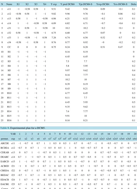
In this section we wish to show, in Table 7, the values of the results of our investigation of the technological property on polypropylene: the first 9 objects are measured experimentally (training set), while the subsequent 16 objects (testing set) show their predictions by the model obtained from the first block. We decided to use the testing set by selecting the extreme points of the domain covered: since we have 4 variables we have an hyper-cube with 16 vertices, ordered according Yates. The results confirm once more that the two models are equiva-lent, but the planning was meant to this end and they are somewhat flat and cannot find significant improve-ments of the response. Data collected on polystyrene (not reported) show exactly the same trend.

The results reported in the first part of Table 7 list the real y values (y exp) of the objects of the training set, and their predictions by each of the two models DCM4 and DCM4-S, i.e. with and without x4, that are very close, thus confirming that x4 does not contribute to the mixture performance.

Columns 10 and 11 list the differences between the experimental and the real data: the larger differences are shown by the objects 4, 7 and 9 (from −0.73 to 0.70), whereas column 12 lists their differences. In order to ex-plore the range of variation outside the experimental design we decided to use as testing set all the extreme points of the domain covered. Since we have 4 variables we have a hypercube with 16 vertices, The second part of Table 7reports the predictions of y for the 16 hypervertices of the 4D space.

On inspecting the training set we find only 3 objects out of 9 with significant difference between experimental and prediction value, so that the model is reliable. However, since all predictions are somewhat similar to the experimental values: this means that the surface model is flat, without sufficient information for finding the way for increasing the technological property. The results confirm once more that the two models are equivalent, but since the planning was meant to this end the models cannot find significant improvements of the response. Also the data collected on polystyrene (not reported) show exactly the same trend.

To help rising the response we can go back to inspect the relationship between y values and the amounts of the x values. The results on the vertices H5, H7, H13 and H15 show that reducing x1 and increasing x3 should increase the response.

6. Extension to DCM5

Table 7. Results for the training and testing sets.

N Name X1 X2 X3 X4 Y exp Y pred DCM4 Ypr.DCM4-S Yexp-DCM4 Yex-DCM4-S Delta

1 e11 −1 −0.58 0.58 1 9.51 9.42 9.56 0.09 −0.1 0.1

2 e12 −0.58 0.58 1 −1 9.82 9.96 9.76 −0.1 0.06 0.2

3 e13 0.58 1 −1 −0.58 6.06 6.21 6.32 −0.2 −0.3 0.1

4 e14 1 −1 −0.58 0.58 6.09 6.82 6.71 −0.7 −0.6 0.1

5 e31 −1 0.58 1 −0.58 10 10.2 10.2 −0.2 −0.1 0

6 e32 0.58 1 −0.58 −1 6.75 6.68 6.77 0.07 0 0.1

7 e33 1 −0.58 −1 0.58 7.26 6.74 6.56 0.52 0.7 0.2

8 e34 −0.58 −1 0.58 1 8.76 8.77 8.92 −0 −0.2 0.2

9 CC 0 0 0 0 8.75 8.24 8.28 0.51 0.47 0

10 H1 −1 −1 −1 −1 8.16 8.19 0

11 H2 1 −1 −1 −1 6.45 6.45 0

12 H3 −1 1 −1 −1 7.5 7.7 0.2

13 H4 1 1 −1 −1 5.8 5.95 0.2

14 H5 −1 −1 1 −1 9.97 9.62 0.4

15 H6 1 −1 1 −1 8.16 7.77 0.4

16 H7 −1 1 1 −1 10.2 10 0.2

17 H8 1 1 1 −1 8.39 8.19 0.2

18 H9 −1 −1 −1 1 8.43 8.21 0.2

19 H10 1 −1 −1 1 6.77 6.45 0.3

20 H11 −1 1 −1 1 8.11 7.7 0.4

21 H12 1 1 −1 1 6.45 5.95 0.5

22 H13 −1 −1 1 1 9.35 9.62 0.3

23 H14 1 −1 1 1 7.6 7.77 0.2

24 H15 −1 1 1 1 9.91 10 0.1

25 H16 1 1 1 1 8.16 8.21 0.1

Table 8. Experimental plan for a DCM5.

VAR 1 2 3 4 5 6 7 8 9 10 11 12 13 14 15 16 17 18 19 20

permut. exp x1 x2 x3 x4 x5 x12 _x22 _x32 _x42 _x52 _{x1x2 x1x3 x1x4 x1x5 x2x3 x2x4 x2x5 x3x4 x3x5 x4x5}

ABCDE e11 −1 −0.7 0 0.7 1 1 0.5 0 0.5 1 0.7 0 −0.7 −1 0 −0.5 −0.7 0 0 0.7

BCDEA e12 −0.7 0 0.7 1 −1 0.5 0 0.5 1 1 0 −0.5 −0.7 0.7 0 0 0 0.7 −0.7 −1

CDEAB e13 0 0.7 1 −1 −0.7 0 0.5 1 1 0.5 0 0 0 0 0.7 −0.7 −0.5 −1 −0.7 0.7

DEABC e14 0.7 1 −1 −0.7 0 0.5 1 1 0.5 0 0.7 −0.7 −0.5 0 −1 −0.7 0 0.7 0 0

EABCD e15 1 −1 −0.7 0 0.7 1 1 0.5 0 0.5 −1 −0.7 0 0.7 0.7 0 −0.7 0 −0.5 0

ACBED f21 −1 0 −0.7 1 0.7 1 0 0.5 1 0.5 0 0.7 −1 −0.7 0 0 0 −0.7 −0.5 0.7

CBEDA f22 0 −0.7 1 0.7 −1 0 0.5 1 0.5 1 0 0 0 0 −0.7 −0.5 0.7 0.7 −1 −0.7

BEDAC f23 −0.7 1 0.7 −1 0 0.5 1 0.5 1 0 −0.7 −0.5 0.7 0 0.7 −1 0 −0.7 0 0

EDACB f24 1 0.7 −1 0 −0.7 1 0.5 1 0 0.5 0.7 −1 0 −0.7 −0.7 0 −0.5 0 0.7 0

DACBE f25 0.7 −1 0 −0.7 1 0.5 1 0 0.5 1 −0.7 0 −0.5 0.7 0 0.7 −1 0 0 −0.7

The strategy applied to DCM5 matrices, i.e. selecting the first submatrix and the most different sequence of the other coded values, gives the needed experimental data to be interpreted in terms of importance of each variable (gamma 1) to modify the y value, i.e. the property under investigation to be maximized or minimized. Details will be reported in a future paper.

Acknowledgements

The authors wish to thank dr. Matthias Henker (Flint Group Germany) for financing a partnership contract with MIA srl, and prof. Svante Wold and his coworkers in Umeå (Sweden) for introducing SC to chemometrics.

References

[1] Clementi, S., Fernandi, M., Decastri, D. and Bazzurri, M. (2014) Mixture Optimization by the CARSO Procedure and DCM Strategies. Applied Mathematics, 5, 3026-3039. http://dx.doi.org/10.4236/am.2014.519290

[2] Clementi, S., Fernandi, M., Baroni, M., Decastri, D., Randazzo, G.M. and Scialpi, F. (2012) MAURO: A Novel Strat-egy for Optimizing Mixture Properties. Applied Mathematics, 3, 1260-1264. http://dx.doi.org/10.4236/am.2012.330182

[3] Clementi, S., Cruciani, G., Curti, G. and Skagerberg, B. (1989) PLS Response Surface Optimization: The CARSO Procedure. Journal of Chemometrics, 3, 499-509. http://dx.doi.org/10.1002/cem.1180030307

[4] Baroni, M., Costantino, G., Cruciani, G., Riganelli, D., Valigi, R. and Clementi, S. (1993) Generating Optimal Linear PLS Estimations (GOLPE); an Advanced Chemometric Tool for Handling 3D-QSAR Problems. Quantitative

Struc-ture-Activity Relationships, 12, 9-20. http://dx.doi.org/10.1002/qsar.19930120103

[5] Clementi, S. and Wold, S. (1995) How to Choose the Proper Statistical Method. In: van de Waterbeemd, H., Ed.,

Chemometric Methods in Molecular Design, VCH, Weinheim, 319-338.

[6] SIMCA 4.01. www.umetrics.com