Why might climate change not cause conflict? an agent based computational response

Why might climate change not cause

conflict? an agent-based computational

response

Hassani Mahmooei, Behrooz and Parris, Brett

Department of Econometrics and Business Statistics, Monash

University, Australia

November 2012

Electronic copy available at: http://ssrn.com/abstract=2172669 Electronic copy available at: http://ssrn.com/abstract=2172669

Why might climate change not cause conflict?

An agent-based computational response

Behrooz Hassani-Mahmooei and Brett W. Parris

Department of Econometrics and Business Statistics, Monash University, VIC3800, Australia

[email protected]

November 2012

Abstract

In this paper, we first briefly review the recent literature on climate change, resource scarcity and

conflict. This is then followed by introducing an agent based computational model based on the

theory of production and conflict which is capable of simulating the dynamics of micro-level

resource conflicts. The model considers differences in resource attributes, differentiates between

conflict subjects, takes into account bounded rationality, nonlinearity and feedback loops, and is

enriched by a set of scenarios ranging between mild to severe resource shocks. Our results show

that agents tend not to get engage in conflict during mild resource scarcity scenarios as they adapt to

the changes and since the decreases in returns to resource predation and increases in their protective

practices act as negative feedback loops, discouraging resource predators from allocating further

effort to predation. The model results also show that scarcity is more likely to encourage product

predation rather than resource predation among the agents.

JEL: Q54, D74, Q34, C61, C63

Keywords: Climate Change, Resource Scarcity, Conflict, Security, Agent-based Model

Electronic copy available at: http://ssrn.com/abstract=2172669 Electronic copy available at: http://ssrn.com/abstract=2172669

1. Introduction

On December 8, 2009, a day after United Nations Climate Change Conference started in

Copenhagen, the Proceedings of the National Academy of Sciences (PNAS) published a paper by

Marshall Burke and his colleagues claiming that the risk of civil war increases in Africa when the

temperature is higher (Burke, et al., 2009). Almost a year later, the same journal published a paper

by Halvard Buhaug (2010a) titled “Climate not to blame for African civil wars”, rejecting the

results of Burke, et al. (2009). Few months later Burke and his colleagues responded to Buhaug’s

paper (Burke, et al., 2010b) which in turn received a response from Buhaug (Buhaug, 2010b).

Sutton et al. (2010) also published a letter in PNAS titled “Does warming increase the risk of civil

war in Africa?”, raising concerns with the findings of Burke et al. (2009) which received a response

later in the same year in an another letter to PNAS (Burke et al., 2010c).

This is not an isolated or unusual exchange since academic debate continues on whether climate

change might initiate new or intensify current conflicts (Salehyan, 2008; Scheffran, et al., 2012).

Several recent studies were reported in the special issue of Journal of Peace Research where Nils

Petter Gleditsch (2012, p.3) concludes: “Overall, the research reported here offers only limited

support for viewing climate change as an important influence on armed conflict.”

The editors of Climate Change, Human Security and Violent Conflict: Challenges for Societal

Stability stated moreover that “climate change has no automatic effect on human security, on

societal stability, or on violent conflict. Rather, there are multiple links in the chain between

changes in the natural environment and these phenomena, which mitigate or multiply the effects of

climate change” (Scheffran et al., 2012, p.797).

This paper attempts to respond to a critical question that we believe has not been addressed

comprehensively so far in the literature: Why, contrary to the theoretical perceptions and

expectations, might climate change and its consequent resource scarcity not lead to conflict and

To respond to this question, instead of investigating case studies or analyzing large-N datasets

which has caused controversy in this area so far, we present a theoretical computational model

based on a well-known economic framework which, borrowing Schelling’s (1978) terms, associates

individuals’ micro-motives with emergent macro-behaviors of conflict.

Next section introduces the unsettled literature on the climate-conflict (CC) link and briefly reviews

the current state of debate. After introducing our theoretical framework and analytical approach, the

model is introduced and its verification and basic outputs are presented. Finally, the scarcity

scenarios and their impacts on the results are discussed, followed by conclusions where we adress

our primary research question.

2. The Debate

The security aspects of climate change have been highlighted by high-ranking policymakers and

institutions. According to the Washington Post (Lynch, 2007), U.N. Secretary-General Ban

Ki-Moon first addressed the U.N. General Assembly on the issue in 2007, stating that future extreme

climatic events such as droughts, floods our constant inundations may lead to scarcity of arable land

and so drive war and conflict0F

1

. In September 2009, New York Times also published Barak Obama’s

speech on climate change at the U.N. General Assembly, warning against “conflict in places where

hunger and conflict already thrive” (Obama, 2009). In July 2011, The Guardian reported on a UN

Security Council meeting discussing the formation of “green helmets” as a peacekeeping force to

act when climate-induced conflicts occur (Goldenberg, 2011)1F

2

.

1

The full statement is available on the UN news centre at:

http://www.un.org/apps/news/story.asp?NewsID=21720&Cr=global&Cr1=warming

2

For further details see: Security Council 6587th meeting documents at:

Researchers are not as confident as politicians, since the issue of resource-driven conflicts has been

source of disagreement, when the impacts of both resource abundance and resource scarcity are

investigated.

In the final years of the last century, two studies, Sachs and Warner (1995) and Collier and Hoeffler

(1998), caused a wave of academic debate by showing how natural resource abundance can lead to

lower levels of economic growth and higher risks of war.

Over the next decade, many studies tried to better investigate the channels which may link resource

abundance to conflict and as time passed more evidence was presented concluding that in the

majority of cases, it is the institutional capacity of a country or a region in managing its natural

resource wealth which determines its growth and security, and not the resource abundance per se

(Ross, 1999; Maxwell and Reuveny, 2000; Mehlum et al. 2006; Brunnschweiler, 2008;

Brunnschweiler and Bulte 2009).

The same story can be observed for resource scarcity. The potential links between resource scarcity

and conflict, especially scarcity driven by climate change, have been discussed widely over the last

couple of decades and almost every paper published in this area over the past few years has briefly

or extensively reviewed how different studies have reached diverse, and sometimes even

contradictory conclusions2F

3

.

For instance, while authors such as Grossman and Mendoza (2003) and Homer-Dixon (1991 and

1994) used theoretical and empirical models to associate resource scarcity and conflict, interestingly,

many recent studies such as Adano et al. (2012), Benjaminsen et al. (2012), Butler (2012) and

Buhaug and Theisen (2012) highlights the social, economic and political institutions as the main

factors affecting the conflict decisions of individuals, communities or states. Raleigh and Urdal

(2007, p.674) concluded that: “political and economic factors far outweigh those between local

3

We avoid repeating the entire literature here since it has been broadly covered by Theisen (2008), Salehyan (2008),

level demographic/environmental factors and conflict”. Nevertheless, there are still studies

published recently, showing how conflict is significantly affected by resource scarcity such as

freshwater availability, land degradation and rainfall (Hendrix and Salehyan, 2012; Urdal, 2008).3F

4

In this paper, we apply a widely-used economic framework, called the theory of Production and

Conflict4F

5

(P&C) and implement it by developing an agent-based computational model to examine

what circumstances in which climate change might or might not cause conflict.

3. Theory and Modeling Approach

The building blocks of production and conflict theory are simple. According to this theory,

economic entities do not merely allocate effort to produce goods and services, but they may also

allocate some unproductive effort to predate others’ resources (raw materilas), final products, rights

and wealth, or protect themselves from being predated by others (Hirshleifer, 1988; Grossman,

1998, 2001).

While these types of models were originally developed to study topics in property rights protection,

later versions were applied to explore issues such as rent-seeking behavior and resource conflicts

(Garfinkel and Skaperdas, 2007; Hausken, 2005; Lahiri, 2010; Muthoo, 2004).

At least three studies have used this framework so far to explore the relations between resource

access and conflict. Grossman and Mendoza (2003) presented an equation-based model of this

theory where they found that resource scarcity, especially when it is transitory leads to further

appropriative competition. Reuveny et al. (2011) developed a game theoretic model based on this

theory and being able to replicate some of the real-world patterns and trends, concluded that

“increasing the resource carrying capacity and growth rate intensifies the fighting” (p.709). Butler

4

Authors such as Hartmann (2010), Brauch (2009) and Oels (2012) have warned against the securitization of climate change. Slettebak (2012, p.163) satates that “one worrying facet of the claims that environmental factors cause conflict is that they may contribute to directing attention away from more important conflict-promoting factors, such as poor governance and poverty.” It has also been claimed that scarcity can even lead to cooperation among stakeholders and provide motivation for innovation in the affected communities (Dinar, 2009, 2011).

5

and Gates (2012) also introduced a model partially based on this theory and showed that conflict is

sensitive to property rights protection asymmetries.

In order to analyze the complexity of conflict decision at the micro and macro level, we have

applied an agent-based model to simulate how individuals interact in an environment where they

can both produce and predate. Agent-based modeling is “the computational study of systems of

interacting autonomous entities, each with dynamic behavior and heterogeneous characteristics”

(Heckbert, et al., 2010, p.40). In economics, this approach is also known as Agent-based

Computational Economics defined by Tesfatsion (2003, p.264) as “the computational study of

economies modeled as evolving systems of autonomous interacting agents.”5F

6

In agent-based models, the computer provides a “flight-simulator-like interface” (Holland, 1992,

p.29) where agents can represent entities such as individuals, communities, firms, cars, agricultural

crops or climatic factors. Each agent is defined based on some features and functions and various

embedded rules which control its actions and reactions. This approach provides the opportunity of

taking into local interactions between heterogeneous autonomous players which can generate

non-equilibrium states which better explain the nature of a system (Epstein, 2006).

Various studies have discussed the advantages of using agent-based models, including being able to

address unsatisfactory features of conventional approaches such as the perfect rationality of the

agents (Axtell, 2000). Agent-based models are highly flexible and so are better able to represent the

“natural description of a system” (Bonabeau, 2002), especially when we want to present the

human-environment relations (Li and Liu, 2008).

Many authors suggest that the conflict analyses should be undertaken at more disaggregated levels.

Allouche (2011) believes that while long-term high-level data, such as international wars datasets,

can provide insights into how scarcity may lead to conflict, moving toward applying short-term data

6

Other definitions and introductory material on ABM are presented by Axelrod (1997) and also the second volume of

Handbook of Computational Economics (Tesfatsion and Judd, 2006), Macal and North (2010), Heath et al. (2009) and

at more disaggregated levels can be more beneficial, especially when food and water security are

studied. This has been echoed by other authors such as Nordås and Gleditsch (2007), Trombetta

(2012), Scheffran et al. (2012), Hendrix and Glaser (2007) and Theisen (2008), who suggest that

local, sub-national, small-scale and less intense conflicts should be taken in to account in CC

analysis6F

7

.

ABMs can also address the data limitation challenges that scholars face in CC research (Buhaug

and Theisen, 2012; Scheffran et al. 2012), by providing the opportunity to run the model under

different scenarios and study a range of possible outcomes.

Moreover, analyzing the associations between climate change and conflict, we are dealing with a

complex adaptive system (Brauch and Scheffran, 2012; Nardulli and Leetaru, 2012; Butler and

Gates, 2012). Following Ramalingam et al.’s (2008) framework of defining a complex system,

different features of complexity can be identified in our model:

Firstly, conflict as discussed in this paper, is an interaction between at least two parties (Hirshleifer,

1988) and so an agent’s decisions will directly and indirectly affect others’ conflict decisions. This

interdependence among system actors may lead to the formation of feedback loops such as violence

leading to further violence (Adano, et al., 2012). Also, as Trombetta (2012) discusses, assigning

deterministic behavior to humans in CC models and then aggregating them, is one of the issues

which needs to be corrected in these types of models since, as Grossman and Kim (2000) and

Reuveny (2011) discuss, the complex outcomes of these models at the macro level emerge from the

interactions among the individuals rather than decisions being aggregated.

Secondly, nonlinear patterns of behavior have been found in at least at two different levels in CC

models. Hendrix and Salehyan (2012) show how there is a nonlinear relation between rainfall and

social conflict in their studied group of countries in Africa and Scheffran et al. (2012) remind us of

7

the “possible tipping points” and “possible critical thresholds” that may exist in agents’ behaviors

that are capable of triggering climate-induced conflicts.

Conflict models also present high dependency on initial conditions and heterogeneity of features.

Beardsley and McQuinn (2009) comprehensively studied the history and characteristics of two

rebel groups in Asia, the Free Aceh Movement (GAM) in Indonesia and the Tamil Tiger

(Liberation Tigers of Tamil Eelam, LTTE) in Sri Lanka and explore how the differences among the

groups led to two totally different outcomes in the aftermath of the 2004 Indian Ocean earthquake

and tsunami.

ABMs have been widely used in modeling conflict, as presented by Rousseau and van der Veen

(2005), Epstein (2002), and Bhavnani and Miodownik (2009) and Hassani-Mahmooei and Parris

(2009, 2013).

4. Model

To ensure that the model is replicable, it is described using the Overview, Design concepts, and

Details (ODD) protocol (Grimm 2006; Grimm, et al., 2010). The associated Unified Modeling

Language (UML) diagrams (Booch, et al., 2005) are also provided as supplementary material.

Among numerous platforms available for implementing an agent-based model, we have used

NetLogo (Wilensky, 1999). Studies have shown that NetLogo is well equipped with the features

necessary for modeling in the social sciences (Blikstein, et al., 2005; Railsback, et al., 2006).

4.1. Purpose

The main purpose of this model is to implement an agent-based environment which is capable of

simulating effort allocation decisions between productive and conflict activities which is then used

to investigate how resource scarcity is likely to affect agents’ effort allocation between production

4.2. Entities, state variables, and scales

The model has four main entities including the agent, the network, the environment and the

resource.

Each agent represents an individual with six main variables. The variable mxage holds the

maximum expected age of the agent. Over time age, which is initially 1, increases and when it

reaches to mxage, the agent leaves child number of offspring and dies. child holds an integer with

uniform distribution which minimum and maximum values are determined based on the population

scenarios. mxage is a normally distributed random value. To associate agents’ allocation decisions

with their heterogeneous attitude, each agent has a variable which determines its risk taking level,

rsktl. When rsktl is higher, agents are more likely to allocate further effort to predation and less to

protection.

Over the simulation, agents select an effort allocation strategy from the pool of strategies. The

strategy is represented using a bit vector [X1 X2 X3 X4], where: X1 stands for a binary variable

representing predation of resource type 1, X2 similarly represents predation of resource type 2, X3

is for product predation and X4 shows whether the agents produces or not. So, if a bit is 1, the agent

allocates effort to that option and if 0, it does not. For example, the [0 0 1 1] strategy means an

agent predates other agents’ products along with producing itself. In the models which have just one

type of resource, the first two bits are combined and the strategy takes the [X1 X2 X3] format. For

simplicity, a strategy like [1 0 1] is presented as S101 from now on.

Agents are connected to each other through an undirected incomplete network where if A is

connected to B, B is connected to A as well. The connection priority is set so that agents will

connect to the agents spatially closer to them. Sensitivity analyses show that while this does not

affect the results, it improves the model interface. The links are fixed and if a link is broken for any

reason the agent will not attempt to establish new links, unless all of them are broken. The average

The environment is a 50 × 50 bounded square grid where each cell is called a patch. Patches all

have the same physical size in the model’s graphical user interface, representing an area able to

accommodate only one agent.

In our model, four different types of resources are studied. Land which represents agricultural land

is a private resource which can be accumulated and stored by the agent over the long-term and be

inherited between generations. Water-D represents a resource such as drinking water which has

only consumption usage. It is a common resource and can be preserved over a predefined short-term.

Water-P on the other hand has similar features to Water-D, but it represents irrigation water since it

yields utility through the production function. Finally, Water-B (water for Both uses) can be directly

consumed and can also be used in the production process.

The resource scarcity scenarios are mainly controlled by two variables: 1) the Duration of the

resource scarcity, D, and 2) the spatial Area which is affected by the resource scarcity, A. We also

allow for single or multiple occurrences of scarcity, the impacts of which are discussed later.

4.3. Process overview and scheduling

The model runs for 25,000 ticks, where each tick is the smallest discrete unit of time in the model.

During a tick there is a non-zero probability of all of the modules of the model being executed at

least once. Model outputs are recorded every 10 ticks and the first 500 observations are discarded

since they are highly affected by the initial conditions, finally leading to 2000 data points. Each

agent goes through seven steps as described below:

1. Measuring Insecurity: During each tick each agent measures the insecurity in its surrounding

environment. Equation 1 shows how insecurity (insec) is measured for the agent i, at each point of

time T, where attkdit-1 shows how intensively the agent i has been attachked predated in round t – 1.

The intensity of predation is the previous rounds is determined by how much effort the predators

1

1 ∑

(1)

In Equation 1, by using ∑ , at every point of time (T), the agent takes into

account his experience of being predated from time = 0 to time = T and measures a weighted

average value of those experiences by giving more attention to more recent incidents. The process is

adjusted using ϑ and σ. This is then taken to a logistic function to provide a nonlinear distribution of

values between zero and one. After calibrating the module, we have selected ϑ = 0.02 and σ = 1.001

based on the life-span of each agent.

2. Allocate resources: Each agent has one unit of effort to allocate during each tick. The first

decision an agent makes is about how much resources it wants to allocate to protection. Equation 2

shows the resources allocated to protection (protn) based on insecurity (insec) and risk-taking level

(rsktl) of agent i at time t.

1 (2)

Considering Equations 1 and 2, agents who are more risk-averse and have been frequently attacked

recently, allocate more effort to protection.

After deciding on the amount of effort to allocate to protection, the agent is left with (1– protn)

units of effort. This will be allocated between production, resource predation and product predation

as shown in Table 1. In this table, the allocation of effort is presented when only one resource is in

the model. If we have two types of resources, there are three steps for dividing the resource

predation effort (rprdn): 1) agents measure how much of the resource of they have, 2) agents

calculate how important each of these resources as a factor in their production function are, and 3)

agents consider the average of both step 1 and step 2. So, each agent at any point of time measures

the comparative benefit of predating Water-B against Land, and also considers how much Land and

Water-B it already owns to decide how it should allocate its resource predation efforts.

Table 1: Effort allocation patterns based on the strategy selected by the agents

Protection

protn

Production

prodn

R-Predation

rprdn

P-Predation

pprdn

S001 insec 0 0 0

S001 insec 1 – protn 0 0

S010 insec 0 1 – protn 0

S011 insec 1 – (protn + predn) 0 (1 – protn) * rsktl

S100 insec 0 0 1 – protn

S101 insec 1 – (protn + predn) (1 – protn) * rsktl 0

S110 insec 0 (1 – protn) / 2 (1 – protn) / 2

S111 insec 1 – (protn + predn) ((1 – protn) * rsktl) / 2 ((1 – protn) * rsktl) / 2

Strategy: SXYZ, where: X = 1 if the agent predates other agents’ resources and 0 if it does not; Y = 1 if the agent predates other agents’ products and 0 if it does not; and Z = 1 if the agent engages in production and 0 if it does not.

insec = Insecurity, protn = Protection, predn = Predation, rsktl = Risk-taking Level

3. Predate resources: Equation 3 is an extended standard success function, showing how the subject

of a particular conflict, such as the resource, is transferred from one agent to another during a

conflict. For a conflict between agents i and j, the transfers from agent i to agent j are a function of

their mutual predation and protection efforts and wealth, where θ is the predation factor and the

relative value of σ and τ determines the effectiveness of the prey’s protective efforts against the

attacker’s predatory effort. Wealth is measured as the accumulation of income.

. . (3)

By including both the allocation options (predn and protn) and wealth (welth), we ensure the

financial powers of the parties are considered as well as their individual effort. Predating resources

takes place before the production in each tick so the stolen resources can be used.

4. Produce: Equation 4 shows a Cobb-Douglas production function, where prodn represents the

effort allocated to production, techy is the technology, spcln is the agent’s degree of specialization

in production, welth is its wealth and resrs is its resources.

Total capital, 1 . , is measured by combining an agent’s access to

technology with its degree of production specialization and its wealth (financial capital). In

Equation 4, α, β and γ are random variables normally distributed in a way to ensure decreasing

returns to production factors for the majority of agents. At the end, prodd will contain the total

amount of goods produced by the agent i at time t.

5. Predate production: The process of predating products is similar to what was discussed for

resource predation, only the objects of predation are the products produced by the prey, rather than

the raw material as in resource predation.

6. Record: Over time, agents continuously observe their output based on different combinations of

strategies and allocation levels and keep records of the strategy which on average yields the greatest

returns, which is called the best strategy (bstry). In other words, bstry, which is initially set to [0 0 0]

or [0 0 0 0], always contains the strategy with the highest outcome resulting from production and

predation.

The learning module is then implemented through three genetic operators: 1) a mutation which

continuously introduces random changes into agents’ strategies, thereby guaranteeing that each

agent tries different strategies while looking for the strategy yielding the highest returns; 2) a

crossover between the parent’s strategy and the child’s strategy which provides strategy inheritance;

and 3) another crossover which occurs between an agent’s most recent strategy and its best strategy

(bstry), implementing the genetic learning process. The probability of each of these operations to

occur is controlled using mutation-rate, inheritance-rate and crossover-rate, respectively.

7- Check age and reproduce: at the final step, agents increase their age by one. If age is equal to

mxage, new agents are born. The offspring select a new random location and inherit their parent’s

4.4. Design concepts

As Grimm et al. (2010, p. 2765) mention, this design concepts section “does not describe the model

per se” but it is an attempt to review the main “characteristics” of the model.

Basic principles: As discussed earlier, the basic principles of actions and interactions in the model

are based on the theory of production and conflict, which shows how effort can be allocated

between productive and unproductive activities.

Emergence: We expect the final resource allocation trends to emerge from individual actions and

interactions rather than simply being the aggregation of micro-level effort allocation decisions.

Adaptation: The adaptive traits in the model can be direct and indirect. One direct adaptation occurs

when agents increase their protection in response to higher predation from their neighbors. Also, in

response to the changes in the environment such as population, technology or resource access,

agents can change their strategy and so their effort allocation patterns, to ensure that they gain the

highest outcome.

Objectives: The main objective of agent is to increase its outcome by taking into account its

personal features such as risk taking level and its neighbors’ and environment’s characteristics.

Learning: As our strategy framework revealed earlier, we have applied three genetic operators to

embed learning in our agent. This allows us to easily change the number of strategies and at the

same time to implement agents with bounded rationality, since they do not reflect on each strategy

at every point of time (Brenner, 2006), but instead search for a better situation over time and are

affected by a random process which manages the mutation and crossover probabilities. The strategy

framework with genetic operator also enables us to have inter-generational learning.

Prediction: The main prediction that the agent does is using a weighted measurement of its history

of being-attacked to form expectations about future insecurity.

Sensing: The agents detect the resource availability in the environment, the number of their

Interaction: The main interaction channel between the agents is through the predation process

where resources or products are transferred between them.

Stochasticity: The probability values for the genetic operators are considered to be random. Also a

random variable is also embedded in the predation function to control the success rate of predation.

Collectives: No collective actions are implemented in the model.

Observation: Two main sets of variables are observed in the model, including the mean efforts

allocated by all agents to each activity, production, resource predation, product predation and

protection and the share of each strategy selected from the pool.

4.5. Simulation Details

The further details of the model, especially the initial conditions and sensitivity analysis are

presented in this section.

The model starts with 25 agents in a 50 by 50 cell environment. The main variables and their initial

values are listed in Table 3. Resources, agents and their children are distributed randomly in the

environment. The land regime is set in a way that the children can not only inherit land, but they

can also gain their own land over time. The mean value of initial resources in each cell is 10 and the

model has only one type of agent.

The Cobb-Douglas production function powers from Equation 4, α, β and γ, are all distributed

normally with mean = 0.3 and s.d = 0.05, which means that less than 10% of the entities experience

constant or increasing returns to scale.

4.5.1 Sensitivity Analysis

We ran a set of sensitivity analysis simulations to select the appropriate initial conditions for some

of the variables. As expected, changes in mutation, optimization and inheritance rates significantly

affect the model outputs since they determine how frequently agents’ bit patterns are updated over

time. High mutation and low inheritance rates increase the stochastic behavior, decreasing the

most beneficial strategy. On the other hand, while frequent optimization can ensure that agents

follow the best strategy, it prevents them from searching for global optimums.

Based on the calibration results and considering each agents’ life cycle, the value of the mutation

rate is set in a way to guarantee, on average, four mutations over its life time. Based on this, the

optimization rate is set to ensure that between each two mutations, on average, ten optimizations are

undertaken. Finally, the value of the inheritance rate is assigned to provide a 50% probability of the

agent following its parent across the whole bit thread.

The predation success rates for both product and resource are 25%. As expected, lower rates of

predation success decrease agents’ interest in attacking others, but since lower predation is a factor

encouraging agents to predate more as others protect themselves less and returns to predation are

high, the success rate impacts are not as high as expected, but still statistically significant.

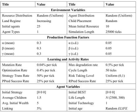
Table 2: Sample initial conditions

Title Value Title Value

Environment Variables

Resource Distribution Random (Uniform) Agent Distribution Random (Uniform)

Land Regime Increasing Child Placement Random

Initial agents 25 Mean Initial Resource 10

Agent Types 1 Simulation Length 25000 ticks

Production Function Factors

α (mean) 0.3 α (s.d.) 0.05

β (mean) 0.3 β (s.d.) 0.05

γ (mean) 0.3 γ (s.d.) 0.05

Learning and Activity Rates

Mutation Rate 0.04% per tick Max degradation rate 0.5% per tick

Optimization Rate 0.4% per tick Cycle Length 50 ticks

Strategy Trans Rate 50% per tick Risk Taking Level Uniform (0,1)

PPred Success Rate 25% per tick RPred Success Rate 25% per tick

Agent Variables

Initial Strategy [0 0 0] Initial BEST [0 0 0]

Average Children 1.5 Life Length N (2500, 300)

Avg. Initial Wealth 5 Initial Technology 1

Agents are each linked to 5% of the population in the environment. The impacts of different levels

of connectivity are mixed. While a higher level of connectivity leads to an increase in the chances

of predating, since the agents have more options to attack, it decreases the probability of one agent

being predated by one specific neighbor over time and these forces neutralize each other and the

changes in connectivity do not significantly affect the model output.

4.5.2. Randomness Sensitivity Analysis

The model is affected by two sets of factors. Firstly, the initial conditions which were reviewed in

the previous section, as well as the random seed which is selected by the software package.

NetLogo uses a pseudo-random number generating system which means that while the random

numbers are “random”, their generation process is deterministic, so choosing the same random seed

in different simulations ensures that the final thread of numbers produced will be the same. As these

differences can affect our results, we checked how sensitive the model is to the random seeds, by

running the model 30 times, each with a different random seed.

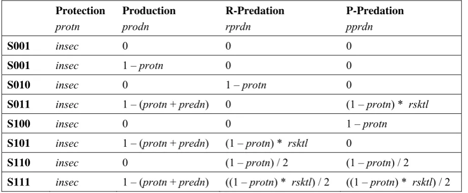
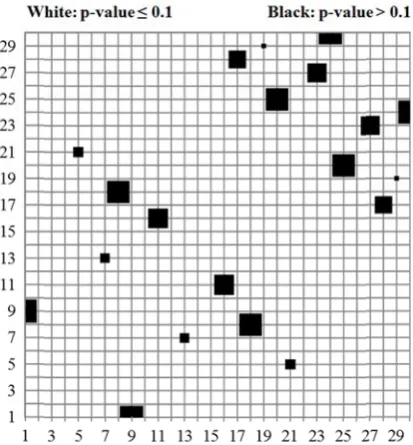
The results are presented in Figure1. Here, there are one line for each x and y coordinate making a

grid line of 900 crossovers when the lines cross. When a x crosses a y line, it produces a black area

if the two seed outputs are statistically significantly different7F

8

. Then, we consider all of these 870

values (900 observations minus 30 of them where a series is compared with itself) as one single

dataset and test if the mean of this sample is more than 0.01 which is rejected at 99% concluding

that there in not enough evidence to claim that the model outputs are significantly different under

different random seeds.

8

Figure 1: On

over the sim

Based on t

initial cond

seeds prov

significant

4.6. Basic

Before pre

scenarios a

scarcity sce

Figure 2 pr

pure produ whether sh and mainly neighbors’ Pure resou having reso ne-to-one sen mulations. H0 these result ditions impo

vides the ch

ly and so th

Model Ver

esenting the

are not act

enarios.

resents the

uct predator

hort-run vol

y result fro

decisions a

urce predati

ources.

nsitivity analy

: Equal mean

s, it can be

osed by dif

hance of ha

he results ca

rification

results, we

tive. This is

variations i

s (S010), or

atilities or l

om how age

and how dif

ion stays cl

ysis results fo

ns of any two

said that th

fferent rando

aving differe

an be analyz

first review

s done to v

in the propo

r pure resou

long-run cy

ents select t

fferent envi

lose to zero

or independe

simulations.

he model is

om seeds. I

ent experim

zed indepen

w a few outp

verify the c

ortion of ag

urce predato

yclical behav

their strateg

ironment va

o, since the

nce from ran

Larger squa

s not signifi

In other wor

ments, it do

ndently.

puts from th

code and a

ents who th

ors (S100) is

vior, are ob

gies based

ariables chan

ere is no dir

ndom seed va

ares show hig

cantly sens

rds, while u

es not chan

he basic mo

also better c

hink being p

s the best st

served in ev

on their pe

nge at the l

rect return

ariations and

gher values.

sitive to cha

using differ

nge the mo

odel where t

clarify the

pure produc

trategy. The

very single

ersonal attri

local and gl

to only pre

equal means

anges in the

Figure 2: Trends of pure production (S001), pure product predation (S010), and pure resource predation (S100).

Regressing the productive allocations against the strategies (excluding the S000), Table 3 shows

that majority of the strategies have significant impacts on the agents’ productive effort allocation

decision. As expected, the pure product predation strategy has the highest negative and the pure

production strategy has relatively the highest positive impact on the productive allocations, while

the dual production-predation strategies have lower or even insignificant effects. The insignificance

of the triple and dual strategies is due to the fact that these strategies, by omitting the protective

efforts, divide the rest of the effort between production and predation and so have unclear impacts

on productive allocations. The insignificant effect of S100 is due to the fact that the strategy is not

practiced by many agents and so its proportion value is close to zero.

Table 3: Productive allocation against the main strategies

Y: Productive Allocation

Durbin-Watson stat 2.087326 Standard Error 0.007744

R Square 0.957432 Observations 2150

Coefficients Standard Error t Stat

Intercept 0.2866 0.05859 4.8932

S001 0.2240 0.0628 3.5654

S010 -0.1945 0.0690 -2.819

S011 0.0985 0.0655 1.5023

S100 -0.0770 0.1055 -0.7304

S101 0.1072 0.0625 1.7131

S110 -0.1670 0.0696 -2.3976

S111 0.0545 0.0646 0.8442

-10% 0% 10% 20% 30% 40% 50%

0 500 1000 1500 2000

Strategy Selection

Time

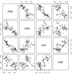
Figure 3 presents the mutual resource allocation patterns between each pair of options. As expected

there is a negative relation between production and each of predation options, and between

protection and production, and both predation options lead to higher levels of protection.

Figure 3: Mutual relations between any two effort allocation options for random observations.

In addition to the presented outputs and also using NetLogo debugging capabilities, each module

was tested separately, to ensure that the intended design is implemented correctly based on a simple

version of what is called abstract interpretation (Hermenegildo, 2005) in computer science, as well

as running the model under two sample agents to ensure correct communications and interactions.

5. Scarcity Models’ Results

The model provides us with an extended set of results which cannot all be presented in the course of

this paper. As a result, we only discuss the major outputs.

5.1. Land Scarcity

In Figure 4 the vertical dash of lines indicate the start and the end of a medium-intensity resource

shock period.

PRD

0.17 0.19 0.21 0.22 0.24 0.26

0.

34

0

.3

8

0.4

2

0

.1

7

0.

1

9

0.

21

PRR

PRT

0

.1

2

0.

14

0

.1

6

0.

18

0.34 0.38 0.42

0.

22

0

.24

0

.2

6

0.12 0.14 0.16 0.18

Figure 4: Changes in the efforts of all agents allocated to product predation (PPred) and percentage of product

predators (S010) in the population in a simulation with medium shock

Two main issues can be seen in the figure. On one hand, during the resource scarcity period, there is

an upward trend in product predation resource allocation, which finishes as soon as the shock

disappears. But this 25% increase in product predation is not unprecedented since as can be seen in

the figure, between times 5100 and 5200 another increase with similar amplitude but shorter time

period is experienced where no scarcity scenario is active. When the model is run under a set of

weak, medium and severe scarcity scenarios and the average of all is measured, at 95% confidence

level, the trends are similar to the models without any scarcity.

To better explore the role of Land shocks in the changes observed in the predatory trend, we

analyze the impulse responses in two different models. First, the model is run with one resource

shock at a predetermined time (t = 1100), while in the second, the model is hit by four shocks (t =

300, 700, 1100, 1400).

Confirming our initial findings, analyzing the impulse impacts shows that in the majority of cases

the changes in the allocation trends are temporary, if not insignificant and according to the results,

less than 5% of the changes in effort allocation patterns can be attributed to the resource shocks.

The model also shows that a single shock is more likely to cause a structural break in the effort

allocation trends, compared to multiple shocks.

R² = 0.7602

5% 10% 15% 20% 25% 30% 35%

5000 5200 5400 5600 5800 6000

Allo

ca

tio

n

Time

To study th

regions as

left side (s

agents loc

environme

In Figure 5

in that area

around 25%

almost 15%

by the sho

considering

effort alloc

Figure 5: C

environmen

which takes

5.2. Water

As introdu

type which

he impacts o

shown in F

shadowed a

cated in ea

ent.

5 each black

a. It is clear

%, in the a

%. The high

ock, but is a

g that in m

cation acros

Changes in t

nt is divided

their resourc

r-D _Scarcity

uced in Sect

h can only b

of Land sca

Figure 5 and

area). The

ach region

k dot shows

r that in a si

affected area

hest rate of p

also the fart

models with

ss the enviro

the product

into 10 regio

ce level to zer

y

ion 4-2, Wa

be consumed 20% 22% 24% 26% 28% 30% Allocated Effort

arcity more p

d the shocks

effort alloc

to see wh

s the averag

imulation w as average predatory e thest region random sho onment. predation ef

ons and only

ro.

ater-D (repr

d directly. F y = -0

% % % % % % 1 2 precisely, th

s were arran

cation patte

hether there

ge effort allo

where the av

product pre

ffort is obse

n from the

ocks, there

ffort allocatio

y four of the

resenting re

Figure 6 sho

.00x3_{+ 0.01x}

R² = 0.

3 4 5

Region

he environm

nged to only

rns were th

e was any

ocated to pr

verage effor

edation is h

erved in Re

unaffected

are no stati

on in a mod

m, the shado

esources suc

ows how an

2_{- 0.05x + 0.3}

.77

6 7 8 9

ns

ment was di

y affect the

hen monito

significant

roduct preda

t allocated t

higher than

gion 1, whi

area. These

istically sig

del with regi

owed area, a

ch as drinkin

n increase in 33

9 10

ivided into

40% of pat

ored separat

t variation

ation by age

to product p

the global

ich is not on

e results are

gnificant dif

ional shocks

are affected b

ng water) is

n the area af

10 different

tches on the

tely for the

across the ents located predation is average by nly affected e important fferences in

. The model

by the shock

s a resource

Water-D shock changes the average proportion of agents who prefer to be pure producers. As can

be seen, when the affected area extends, more agents decide to leave the pure production strategy

and become predator by enabling their predation bit.

Figure 6: The final value for the proportion of pure producers in simulations with different levels of affected

areas affected by the shock.

To analyze the shock thoroughly, a set of impulse response tests was undertaken for all six main

strategies (leaving out S000 and S100) to investigate the short- and long-run impacts of the shocks,

at different levels of scarcity. Table 4 contains the results for these tests.

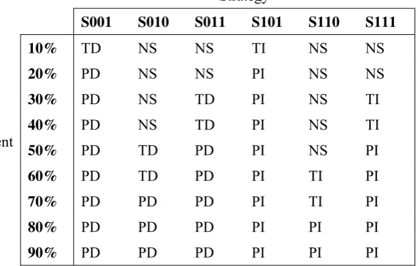
Table 4: Agent populations’ selection of different strategies in reaction to the Water-D shocks for different

spatial extents. NS = Not Significant, TD = Temporarily Decreasing, TI = Temporarily Increasing, PD: =

Permanently Decreasing, PI = Permanently Increasing.

Strategy

S001 S010 S011 S101 S110 S111

Shock Extent (% of area)

10% TD NS NS TI NS NS

20% PD NS NS PI NS NS

30% PD NS TD PI NS TI

40% PD NS TD PI NS TI

50% PD TD PD PI NS PI

60% PD TD PD PI TI PI

70% PD PD PD PI TI PI

80% PD PD PD PI PI PI

90% PD PD PD PI PI PI

y = -9E-05x4_{+ 0.0023x}3_{- 0.0174x}2_{+ 0.0032x + 0.3268}

R² = 0.9999

0% 10% 20% 30% 40%

A-10% A-20% A-30% A-40% A-50% A-60% A-70% A-80% A-90%

Allo

ca

tio

n

As the table suggests, at the lower levels of shocks the producer agents (SXX1) temporarily switch

from just producing to predating Water-D as well as producing. At 20% level of shock, a similar

impact is found, but this time it is permanent since a bigger group of agents experience the shock.

As the shocks become more extensive the second group of non-resource-predating agents (S0XX)

gradually joins the formerly-pure producers, by first temporarily and then permanently allocating

effort to predating others’ resources. The results show that after the shock level passes 50% of the

area, almost all non-resource-predating agents are affected, since they attack others to gain Water-D

and survive. This becomes permanent when the shock is at its full extent, so model responses

changes in the long term changes.

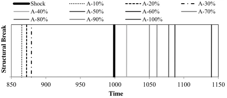
To identify possible structural breaks, the Chow test is applied to the allocation trends. As presented

in Figure 7, low intensity scenarios do not cause any breaks immediately after the shock, while

when the shocks become severe, the model responds by a significant change in the output trends.

Figure 7: Shock and structural breaks in a sample run with Water-D as the resource - single run.

While the severe scarcity of a resource such as Water-D should lead to severe consequences for the

agents, such as death, we did not allow the agents to die due to resource scarcity in the initial model

in order to be able to follow the dynamics of their strategy selection over time. When we relax that

constraint allowing the extremely thirsty agents die after passing a pre-defined threshold, the

population trends react as shown in Figure 8. As the figure shows, while Water-D scarcity does not

0.1

850 900 950 1000 1050 1100 1150

Structural Break

Time

Shock A-10% A-20% A-30%

A-40% A-50% A-60% A-70%

affect population trends at low or medium levels of shock intensity, at higher levels the population

drops very fast during the simulation.

Figure 8: Final population and affected area in a Water-D _{model with death – 30 runs}

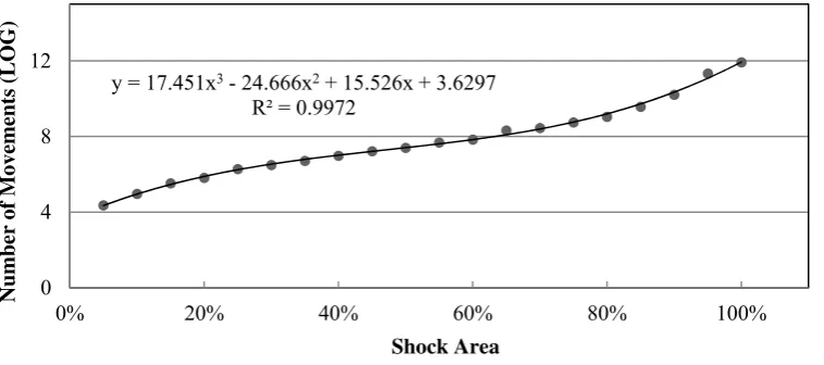
We relax another limitation by allowing the agents to move in response to Water-D scarcity,

searching for resources in the environment. As can be seen in Figure 9 where the natural log of the

number of movements is presented against the affected area, the number of movements increases

exponentially as a result of increasingly severe resource scarcities.

Figure 9: Changes in the number of moves in the model based on the different levels of scarcity – Multiple run.

Migration is an effective strategy also as Figure 10 shows, in the models with the migration option

active (white boxplots), the effort allocated to productive action has decreased less due to different

extents of shock, compared to the equivalent cases where migration is not allowed (grey boxplots).

y = -0.2454x4_{+ 4.3622x}3_{- 27.212x}2_{+ 68.455x + 148.14}

R² = 0.9882

0 100 200

Population

Area Affected

y = 17.451x3_{- 24.666x}2_{+ 15.526x + 3.6297}

R² = 0.9972

0 4 8 12

0% 20% 40% 60% 80% 100%

Number of

Movements

(LOG)

Figure 10: Decreases in productive allocation when migration is active (white) and inactive (grey).

5.3. Water-P Scarcity 

Figure 11 shows how allocation trends react to a Water-P (such as water for production) scarcity

scenario. As can be seen, during the shock, productive efforts are replaced by product predation,

which increases gradually when the shock starts and to a large extent disappears after the shock

finishes. As for the strategies, the significant increases in S010 (product predation) and S011

(product predation and production) are considerable, while effort allocated to the pure productive

strategy falls when the shock starts and returns to its top position when the shock fades out.

Figure 11: Changes in a sample individual-run effort allocation due to Water-P shock – single run.

Figure 12 shows how different levels of resource shock can affect the average proportion of effort

allocated to production in a model with Water-P as the resource.

MA1000 MA2000 MA3000 MA4000 MA5000 MA6000 MA7000 MA8000 MA9000

30

40

50

6

0

A

ll

o

ca

te

d E

ff

o

rt

(

p

er

ce

nt

a

g

e

)

5% 15% 25% 35% 45%

500 700 900 1100 1300 1500 1700 1900

Allocation

Time

As can be shocks, ch shocks bec efforts whe According allocated t overall resu product pr considering

time and so

We have a

If there ha

give the s

moving av

Figure 12:

seen, the p

anges to alm

come longe

en the basic

to the resu

o product p

ults show th

redation, si

g the fact t

o agents nee

also tested f

s been a bre

cenario a s

verage of the 2 2 2 3 3 3 Allo ca tio n

Changes in t

productive

most 30% i

er and affec

c scenario is

ults, the de

predation, s

hat as for L

nce the ret

that Water,

ed to consta

for the exist

eak immedi

score of 1,

e data. 15% 30% 25% 27% 29% 31% 33% 35% Shock Area 27%

the average p

allocation w

in less inten

ct a larger

s compared

crease in th

ince further

and, resour

turns to res

as a comm

antly allocat

tence of a s

iately within and otherw 45% 60% 75% a -29% 29% productive eff which was

nse shock sc

area. The

with very s

he producti

r resource p

rce shocks t

source pred

mon resourc

te effort to i

structural br

n 100 ticks

wise 0. Th

% ₄₀₀

5000

%-31% 31

forts in Wate

more than

cenarios, th

results show

severe shock

ive efforts m

predation is

o Water-P s

dation decr

e in this m

its predation

reak in the m

after the sh

e tests wer 3000

00 Sh

%-33% 33

r-P shocks m

35% in the

en to slight

w a 25% d

ks.

mainly lead

s not efficie

shift the eff

rease due to

odel, canno

n.

model outpu

hock at 99%

re undertak 1000 2000 hock Duration 3%-35% multiple run.

e basic mod

tly over 25%

decrease in

d to more e

ent for the a

fort from pr

to the shoc

ot be stored

uts over the

% confidenc

ken using th 0

n

del without

% when the

productive

effort being

agents. The

roduction to

ck and also

d for a long

e scenarios.

ce level, we

Figure 13: T

area with va

Figure 13

increases a

less extens

in the effo

we did no

occurrence

5.4. Water

Figure 14

resource fo

impacts of

produce or

and produc

while prod

Testing for t

alue of 1, show

shows that

as well. In th

sive areas, b

ort allocation

ot find any

e.

r-B Scarcit

(top) illustr

for both co

f shock dur

r not. The

ct predation duct predatio Sh k D ti he existence

ws scenario c

t as the sho

he results, n

but with lon

n patterns b

y clear rela

ty

rates how p

nsumption

ration and a

middle and

n trends rea

on increases D1000 D2000 D3000 D4000 D5000 A Sh oc k D ura ti on of structura combinations ocks becom no structura

nger and mo

becomes mo

ation betwe

roductive e

and produ

area have s

d bottom pa

ct to the sca

s at high lev 0 0 0 0 0 1500 A3000

al break due

s which have

me more pow

al breaks are

ore extensiv

ore likely. D

een the sho

efforts decli

uction, Wate

significant

anels respec

arcity. Reso

vels of shoc

0 A4500 A

Shock Are

to Water-P _r

caused a stru

werful, the

e experience

ve shocks t

Despite test

ock intensi

ne due to r

er-B. As ca

effects on ctively show ource preda ck intensity. A6000 A7500 ea resource shoc uctural break probability

ed for limite

he existenc

ting for diff

ty and the

esource sho

an be seen

the agents’

w how avera

ation does n

0 A9000

ck scenarios.

k.

y of a struc

ed shock du

ce of a struc

fferent scena

e timing of

ocks in a m

n, again the

’ decisions

age resourc

no change s

. The dashed

ctural break

urations and

ctural break

ario setups,

f the break

model with a

Figure 14: Resource Pr Changes in redation; Bot Shoc Allo ca tio n Sho Allo ca tio n Shock Allo ca tio n effort alloca ttom: Produc 10 00 20 00 40% 45% 50% 55% ck Duration 10 00 20 00 15% 20% ock Duration 30 00 40 00 50 00 k Duration

ation due to

t Predation 30 00 40 00 90% 40%-45% 30 00 40 00 90% n 20 00 30 00 15% 15%-20%

Water-B _re

60 75% % 45%-50% 60 75% % 15%-20% 30% 45% 20%-25% esource shock 45% 0% Shock A % 50%-55% 45% 0% Shock Are % 60% 75% Shock Are % 25%-30%

ks. Top: pro

As we presented in previous cases, applying the impulse response tests shows that the impacts are

only significant when severe shocks affect the model.

5.5. Land and Water-B Scarcity

To measure the possible impacts of parallel Land and Water scarcities on how agents allocate their

efforts, different scenarios were designed based on low-, medium- and high-intensity Land and

Water scarcity combinations. The model was then run 30 times and the average results over

different random seeds were calculated separately for every scenario.

According to the results, when the productive effort allocation is regressed against the scarcity of

each resource, the coefficients are 0.004 and 0.003 for Land and Water, respectively. While the

closeness of the values can be attributed to the fact that both resources, on average, have similar

roles in linking the production function to scarcity, the larger coefficient of Land can be attributed

to the agents’ abilities to preserve their Land over time, which makes its predation more desirable.

Figure 15 shows how the productive allocation effort coefficients are distributed for Water and

Land over the 54 scenarios. As can be seen, while the Land coefficient distribution is close to a

normal distribution, the Water coefficient distribution is skewed. This shows that while Land, on

average, contributes more to the production process in this model, its role in production is less

sensitive to the scenarios, compared to Water which can generate utility via either predation or

consumption.

Figure 15: Distribution of regression coefficients for Land and Water

0 10 20 30

0 0.001 0.002 0.003 0.004 0.005 0.006 0.007 0.008 0.009 0.01

Frequency

Coefficient

Individual regressions for each of the strategies were run against Water-B and Land levels in the

model. The results are presented in Table 5.

Table 5: Strategy selection changes resulting from Land _and Water _{variations. Dependent variable = strategies,}

e.g. S0001 = f (Land, Water). SWXYZ: W: Water-B, X: Land, Y: Product Predation and Z: Production.

SWXYZ Land Water R2 SWXYZ Land Water R2

S0000 N/A N/A N/A S1000 -0.00067

(-47.8874)

-0.00085

(-11.5988) 0.590902

S0001 0.00349

(70.63291)

0.002721

(10.4183) 0.739972 S1001

-1.5E-05 (-0.66624)

-0.0021

(-17.178) 0.131499

S0010 -0.00083

(-55.9514)

0.000227

(2.894349) 0.597578 S1010

-0.00095 (-65.549)

-0.00067

(-8.74781) 0.707277

S0011 0.000987

(40.40638)

0.001007

(7.797153) 0.493947 S1011

0.000439 (17.46697)

-0.00041

(-3.07252) 0.117016

S0100 -0.0002

(-18.6174)

-0.00012

(-2.12893) 0.160524 S1100

-0.00025 (-19.3265)

-0.00094

(-13.8646) 0.284082

S0101 -0.00017

(-6.96071)

0.001391

(10.97296) 0.048042 S1101

-0.00086 (-44.0739)

-0.00116

(-11.3017) 0.554038

S0110 -0.00044

(-29.5389)

-0.00028

(-3.49163) 0.325794 S1110

-0.00057 (-36.5186)

-0.00089

(-10.724) 0.470349

S0111 0.000195

(7.560805)

0.002493

(18.31933) 0.203077 S1111

-0.00027 (-8.84087)

-0.00055

(-3.33685) 0.053989

According to the results, the pure production strategy, S0001, is significantly correlated with Land

and Water access, enjoying the highest levels of significance and R2. This clearly shows that the number of producers decreases due to resource scarcity in the model. Pure product predation is

negatively correlated with Land and positively with Water since Water scarcity shift efforts to

resource predation rather than product predation. The positive, statistically significant and highly

correlated coefficients for S0011 (production and product predation) illustrate the fact that during

the time of scarcity, since production levels fall, there may not be enough incentives for agents to

predate what others have produced, and it can also be due to the fact that this strategy is not capable

Pure resource predation strategies, S0100, S1000 and S1100, all increase due to scarcity, but since

Land cannot generate utility individually, the R2 is much higher for the cases where Water

predation is included in the strategy, S1XXX.

Two more interesting findings can be observed in Table 5. First, S1010, or Water and product

predation has a significant negative correlation with both Land and Water access. It seems that

during times of scarcity, agents prefer to predate Water and the final product to survive, rather than

Water and Land and produce themselves. The coefficients of S1101 (predating both resources and

producing) and S1110 (predating both resources and product predation) are comparatively high,

indicating that resource predation that is accompanied by either production or product predation

seems to be a popular strategy when resources get scarcer.

6. Discussion and Conclusions

It is widely believed that induced resource scarcity is the main factor causing

climate-driven conflicts. Applying the theory of production and conflict and using agent-based modeling

enabled us to address three challenges that have been highlighted in the literature. First, following

the suggestions by many researchers in this field, we applied disaggregated analysis to investigate

the possible links between climate change and conflict. Secondly, we addressed a challenge

highlighted by studies such as Theisen et. al (2011) and Scheffran et al. (2012) as we considered

different levels of intensity for resource scarcity. Finally, we took into account the complexities

involved in modeling conflict which arises from the interactions, feedback loops, thresholds and

nonlinearities which exist when conflict decisions are made.

In line with empirical studies such as Theisen (2008) and Raleigh and Urdal (2007), which claim

that only high or very high levels of land and water scarcity are likely to cause conflict, we showed

that while low levels of scarcity does not affect the effort allocation patterns significantly and

scarcity be trends beco Our findin the historic short-term economic o Figure 16 producer a

while in al

changes in

can be ide

resource sc

increases a

allocate eff

Figure 16: S

without reso 0% 10% 20% 30% 40% 50% 60% 70% 80% 90% 100% Shock Area 0%-ecomes seve ome substan

gs on the li

cal patterns

climatic ev

or political

(left) summ

agents in the

most 50% o

n strategy se

entified. Ba

carcity and

as the resou

ffort to preda

Share of pure

ource scarcity % % % % % % % % % % % -25% 25%

ere, in dura

ntial, since m

inks betwee s McMicha vents, mediu challenges. marizes our e populatio

of the cases

election patt

ased on ou

conflict, a

urce shocks

ating others

e producers d

y.

Shock Du

%-50% 50

ation, spatia

many agent

en the durati

ael (2012) h

um- and lon

r results in

n are shown

(the dotted

terns, in the

ur results, w

s presented

s become m

s rather than

due to differen uration

0%-75% 7

al area or af

ts develop p

ion of scarc

has reviewe

ng-term cha

a sample

wn based on

d area), reso

e other half

we believe

d in Figure

more severe

n producing

nt levels of re

75%-100%

ffected popu

predatory be

city and the

ed: while so

anges are m

case where different le ource scarcit f, significan that there 16 (right),

due to high

g. esource shock Scarcity ulation, the ehavior. likelihood ocieties can

more likely t

e decreases

evels of sca

ty does not

t levels of d

is a nonlin

where the

her portion

ks compared

becomes mo

e impacts on

of conflict

n adapt to

to cause soc

in the sha

arcity. As c

lead to any

decrease in

near relatio

probability

n of agents

to the basic m

ore severe

n allocation

also follow

“recurring”

cial, health,

are of

pure-an be seen,