On the Local Power of Fixed T Panel Unit Root Tests with Serially Correlated Errors

Munich Personal RePEc Archive

On the Local Power of Fixed T Panel

Unit Root Tests with Serially Correlated

Errors

Karavias, Yiannis and Tzavalis, Elias

December 2012

Online at

https://mpra.ub.uni-muenchen.de/43131/

On the local power of …xed T panel unit root tests

with serially correlated errors.

Yiannis Karavias

and Elias Tzavalis

a

:

School of Economics, University of Nottingham

b

:

Department of Economics, Athens University of Economics & Business

Working Paper

December 2012

Abstract

Analytical asymptotic local power functions are employed to study the e¤ects of general form short term serial correlation on …xed T panel data unit root tests. Two models are considered, one that has only individual intercepts and one that has both individual intercepts and individual trends. It is shown that tests based on IV estima-tors are more powerful in all cases examined. Evenmore, for the model with individual trends an IV based test is shown to have non-trivial local power at the natural pN

rate.

JEL classi…cation: C22, C23

Keywords: Panel data models; unit roots; local power functions; serial correlation; incidental trends

a:Yiannis Karavias: [email protected]

1

Introduction

Panel unit root test statistics assuming …xed (…nite) time dimension (T) and large cross-sectional dimension (N) have received much interest in the literature over the last decade, since they can be applied to short panels. Early contributions in this area include Sargan and Bhargava (1983), Breitung and Meyer (1994), Harris and Tzavalis (1999, 2004), Kruininger and Tzavalis (2002), Hahn and Kuersteiner (2002), Bond et al (2005), Kruiniger (2008), Hahn and Phillips (2010) and De Blander and Dhaene (2011). These papers derive the limiting distribution of the suggested tests under the null hypothesis of a unit root in all individual series of the panel. Despite the plethora of studies for the distribution of large-T

panel unit root tests under local alternatives1_{, only recently there has been some interest to}

do so in the literature for …xed-T tests.

Speci…cally, for the AR(1) model with individual intercepts, Bond et al. (2005) derive the limiting distributions, under local alternatives, of the Breitung and Meyer (1994) test, the Harris and Tzavalis (1999) test, the …rst di¤erenced MLE test of Kruiniger (2002) and Hsiao et al. (2002) and the …rst di¤erenced and system GMM of Arellano and Bond (1991) and Blundell and Bond (1998). Kruiniger (2008) also derives the distribution under local alternatives for the …rst di¤erenced MLE in the same model. Madsen (2010) compares the local power functions of the pooled OLS test, the Breitung and Meyer (1994) test and the Harris and Tzavalis (1999) test under alternative assumptions about the initial conditions.

The main purpose of this paper is to derive analytically the limiting distribution of panel unit root tests allowing for serial correlation under local alternatives and, then, to study the asymptotic power properties of these tests. In this framework. This can shed light on how higher order dynamics, or serial correlation of the error term, can a¤ect the local asymptotic power of panel unit root tests and, thus, to choose the best (in terms of power) testing procedure in practice. These e¤ects are studied through Monte Carlo simulations, but not analytically (see De Blander and Dhaene (2011), for panels, and Schwert (1989), for single time series, respectively). The paper consider two …rst order autoregressive panel models: the …rst one has individual speci…c intercepts and the second one has individual speci…c intercepts and individual speci…c trends. Since the model with trends has not been considered in the …xedT literature, one of the aims of the paper is to discuss the "incidental trends" problem of Moon and Phillips (1999).

The present study makes several contributions. First, for the model with individual intercepts, the panel unit root tests of De Wachter et al. (2007) and Kruiniger and Tzavalis (2002) are reformulated and have their local power function analytically derived. De Wachter et al. (2007) propose a panel unit root test based on an IV estimator while Kruiniger and

1_{See, e.g., Moon and Phillips (1999), Breitung (2000), Moon and Perron (2004), Moon et al. (2007),}

Tzavalis (2002) propose a test based on the WG estimator. Analytical local power functions are derived for general forms of short term serial correlation up to orderT 2:In the context of an MA(1) model for serial correlation it is shown that the IV test is always more powerful than the WG test although their behaviour is signi…cantly di¤erent due to the the di¤erent ways that the two tests use the available moments. In both cases positive values of the moving average help power while negative values reduce it. In contrast to the IV test, the WG test becomes biased for large negative values of the parameter. The order of serial correlation has a signi…cant impact on the IV test but not on the WG. Monte Carlo results show that the asymptotic theory provides very good small sample approximations.

Second, for the model with individual trends, the local power for the corresponding test of Kruiniger and Tzavalis (2002) is derived, denoted henceforth as WG*. When there is no serial correlation the test has trivial power as would be expected by the "incidental trends problem". When there is serial correlation, it is shown that the test has power in the natural root-N neighbourhood of unity. In an MA(1) context, positive serial correlation reduces the power of the test and negative increases it; this is the opposite of the case where the model contains only individual e¤ects. An attempt is made to …nd more powerful tests for this case by proposing two new tests: a …xed-T version of the Breitung (2000) test, called henceforth FOD due to the forward orthogonal deviations matrix involved, and an extension of the De Wachter et al. (2007) test for the case of individual trends, called double di¤erence IV test (DDIV) henceforth. It is shown that the …xed-T version of the Breitung (2000) test behaves as the WG* test having in general smaller power or bias, depending on the moving average parameter, and trivial power when there is no serial correlation. The DDIV test is shown to have non-trivial power even in the case when there is no serial correlation. In the MA(1) context it is shown to behave like the IV test of De Wachter et al. (2007). Monte Carlo experiments show that asymptotic theory provides moderate approximations for this case.

The paper is organized as follows: Section 2 introduces the models and the assumptions required for the derivation of asymptotic results. Section 3 derives the asymptotic local power functions and provides results on the behaviour of the tests. Section 4 compares the statistical properties of the two tests. Section 5 conducts a small Monte Carlo experiment con…rming the analytical results and Section 6 concludes the paper. All proofs are relegated to the Appendix. In the following we name the main diagonal of a matrix as "diagonal 0";

2

Models and Assumptions

Consider the following …rst order autoregressive models with individual e¤ects:

M1 : yi ='yi 1+ (1 ')aie+ui; i= 1; :::; N: (1)

M2 : yi ='yi 1+ (1 ')aie+' i+ (1 ') i +ui: (2)

where yi = (yi1; :::; yiT)0 and yi = (yi0; :::; yiT 1)0 are (T X1)vectors, ui is the error term

and ai and i are the individual speci…c coe¢cients of the deterministic components. The

(T X1)vectore has elementset= 1 for t= 1:::T and t=t the time trend. The asymptotic

distributions of the tests are derived under the assumptions:

Assumption 1: (1.1)_fuig is a sequence of independent normal random vectors with

E(ui) = 0; E(uiu0i) = st where is of unknown form apart from i;1T = i;T1 = 0 and

that at least one tt 6= 0 for t = 1; :::; T: (1.2) tt >0 for at least one t = 1; :::; T: (1.3) The

4+ thpopulation moments of yi; i = 1; :::; N are uniformly bounded i.e. for everyl 2RT

such that l0_{l = 1; E(jl}0 _y

ij4+ ) < B <+1 for some B where is the di¤erence operator.

(1.4)l0_{V ar(vec( y}

i y0i)l >0for everyl 2R0:5T(T+1) such thatl0l = 1:(1.5) V ar(yi0)<+1:

Assumption 2: The following hold: E(uitai) = 0; E(uit i) = 0 and E(uityi0) = 0 for

t= 1; :::; T and i= 1; :::; N:

Condition (1.1) restricts the order of serial correlation to be at mostT 2:This condition can be strengthened to allow for smaller orders of serial correlation. Condition (1.2) imposes …nite fourth moments on the initial conditions, the error terms and the individual e¤ects. Along with conditions (1.3) and (1.4) they allow application of the Markov LLN and the Lindeberg -Levy CLT and ensure that all quantities in the denominators are non-zero.

The original WG and IV tests allow for heterogeneous disturbances across i but this assumption is trimmed so that tractable results may be obtained. For the same reasons, normal errors provide analytic formulas for the variances of the tests. Condition (1.1) ensures the existence of at least one moment condition free of correlation nuisance parameters but does not specify the true order of serial correlation. De…ne p the order of serial correlation assumed by the researcher andp the true order. As long asp p the limiting distribution of the test statistics is valid. Since inference in both tests is based on moments that are free of correlation parameters, choosing p > p means selecting fewer than possible moments for inference. For a discussion on how to estimate the order of serial correlation see Hayakawa (2010).

De…ne '_N = 1 _pc

N: Then the hypothesis of interest is:

H0 : c= 0 (3)

where cis the local to unity parameter. Assumption 2 is only required when c >0:

The only assumption on the initial condition is (1.5). Bond et al. (2005), Kruiniger (2008) and Madsen (2010) assume covariance stationary initial conditions which means that

V ar(yi0) =

2

1 '2

N: Then, as N diverges, 'N ! 1 and V ar(yi0) ! +1: This assumption is

not appropriate because it is not plausible that the variance of the initial condition increases with the number of cross section units, see also Moon et al. (2007). All tests in the paper are invariant to the initial condition. The IV, FOD and DDIV tests subtract the initial values of the individual series of the panel from their levels, across all units of the panel2_{. This is}

done for all time-series observations of the panel. The WG tests, for both models become invariant to the initial conditions of the panel by relying on the "within” transformation of its individual time series3_.

To study the asymptotic local power of the tests we employ a "slope" parameter, denoted as k;which is found in functions of the form

(za+ck)

where is the standard normal cumulative distribution function and za the level

per-centile. Since is strictly monotonic, for the samec; a largerk means greater power. Thus, it su¢ces to compare cases by comparing their k, instead of having a visual inspection of the power function. If k is positive then the test has non-trivial power, if it is zero it has power0:05and if it is negative the test is biased.

3

Asymptotic local power functions

This section presents all tests that are studied and derives their asymptotic local power functions. The …rst half is dedicated to model M1and the second to model M2:

3.1

Individual intercepts

IV panel unit root test: De Wachter, Harris and Tzavalis (2007) propose a …xed-T

panel unit root test based on the IV estimator where in a …rst step they subtract the initial observations from all series as in Breitung and Meyer (1994). The test exploits moments of

2_{This approach is suggested by Schmidt and Phillips (1992), for single time series, and Breitund and}

Meyer (1994).

3_{This transformation means that one subtracts the means of the individual series of the panel from their}

the form:

E

"_{T p 1} X

t=1

zitui;t+p+1(') #

= 0; i= 1; :::; N: (5)

and is based on the estimator:

^

'IV = N

X

i=1

T p 1

X

t=1

zitzit+p

! 1 _N

X

i=1

T p 1

X

t=1

zitzit+p+1 !

(6)

where zit =yit yi0:These moments can be rewritten in matrix notation as:

E(z0

i 1 pui) = 0: (7)

where p is a (T XT) matrix that selects the appropriate moments according to equation

(5) and zi 1 =yi 1 yi0e. p has ones in the pth diagonal and zeros everywhere else. The

estimator in (6) can be rewritten as:

^

'_IV = (

N

X

i=1

z0

i 1 pzi 1) 1(

N

X

i=1

z0

i 1 pzi) (8)

The asymptotic distribution of the IV test is given in the following theorem:

Theorem 1 Under Assumptions 1, 2, the assumption that the order of serial correlation is

at most p and as N _{! 1}:

p

N(^'_IV 1) ^V

1 2

IV d

!N( ckIV;1) (9)

where

kIV =

1

p

VIV

(10)

and VIV = 2tr((AIV )

2

)

tr( 0 _{p )}2; AIV =

1

2( 0 p+ 0p ):

Theorem 1 nests both the null and the local alternative hypotheses. For c = 0 (9) presents the distribution of the test under the null as found by De Wachter, Harris and Tzavalis (2007). Result (10) shows explicitly how local power depends on a)the assumed order of serial correlation through matrix p and b)on the form of serial correlation found in

matrix : The test of Breitung and Meyer (1994) can be seen as a special case of the IV test for p= 0: Also, as Bond et al. (2005) show, this can be also seen as a maximum likelihood estimator.

for inference. De…ne the annihilator matrix Q = IT e(e0e) 1e0 where IT is the (T XT)

identity matrix. Then '^W G is de…ned as:

^

'_{W G} = (

N

X

i=1

y0

i 1Qyi 1) 1(

N

X

i=1

y0

i 1Qyi) (11)

The test and its asymptotic distribution under Assumption 1 and as N _{! 1}:

p

N V

1 2

O ^(^'W G 1

^_bO ^_O)

d

!N(0;1) (12)

where:

^_bO ^_O =

vec(Q )S(1 N

N

X

i=1

vec( yi y0i))

1 N

N

X

i=1

y0

i 1Qyi 1

and (13)

VO = vec(Q )0(IT2 S)V ar(vec( y_i y0

i))(IT2 S)vec(Q ): (14)

^ bO

^_O is an estimator of the asymptotic bias of '^W G given as

tr( 0_{Q )}

tr( 0_{Q )} since

^

bO = vec(Q )S

1

N

N

X

i=1

vec( yi yi0)

!

p

!tr( 0_{Q ) and (15)}

^_{O =} 1

N

N

X

i=1

y0

i 1Qyi 1

p

!tr( 0_{Q ) (16)}

whereIT2 is the(T2XT2)identity matrix andS is a(T2XT2)diagonal selection matrix with

elements sij de…ned as s(i 1)T+j;(i 1)T+j = 1 d( ji = 0) with i; j = 1;2; :::; T and d(:) is

the Dirac function. In the above, ^bO

^_O is an estimator of the asymptotic bias of '^W G: is

a deterministic matrix given in the appendix. S is an interlayer matrix in^bO which selects

only the elements of _N1

N

X

i=1

vec( yi yi0)which are nonzero, thus maintaining the consistency

of ^bO and on the same time avoiding the equality between ^ bO

^_O and '^W G 1 which would

deprive the test of any variability:Notice in equations (13) and (14) that the bias correction terms a¤ect both the mean and the variance of the test.

The reformulation avoids the (T2_XT2_{) matrix S employed in the original test because}

(T2_XT2_{)matrices are far more demanding in computational power even for moderate values}

of T. A new selection matrix p;W G is employed which is (T XT)-dimensional having in

else4_{. Then}

tr( p;W G^) = vec(Q )S

1

N

N

X

i=1

vec( yi yi0)

!

(17)

2tr((AW G )2) = vec(Q )0(IT2 S)V ar(vec( y_i y0

i))(IT2 S)vec(Q ) (18)

where

^ = 1

N

N

X

i=1

yi y0i; (19)

a consistent estimator of under the null because yi =uiandAW G = 1₂( 0Q+Q p;W G

0

p;W G):The following theorem provides the limiting distribution of the reformulated statistic

for c 0 :

Theorem 2 Under Assumptions 1, 2, the assumption that the order of serial correlation is

at most p and as N _{! 1}:

p

NV^

1 2

W G^(^'W G 1

^_b ^)

d

!N( ckW G;1) as N !+1: (20)

where

kW G =

tr( 0_{Q ) +tr(F}0_{Q ) tr(}

p;W G ) tr( 0 p;W G )

p

2tr((AW G )2)

: (21)

and '^_{W G} = (

N

X

i=1

y0

i 1Qyi 1) 1(

N

X

i=1

y0

i 1Qyi);

^ b

^ =

tr( p;W G^) 1

N

PN

i=1yi;0 1Qyi; 1 , F =

d

d' j'=1 where

is given in the appendix. The variance is given by VW G = 2tr((AW G )2) where AW G = 1

2( 0Q+Q p;W G 0p;W G). The proof is given in the appendix.

The annihilator matrix Q and the inconsistency correction estimator based on p;W G

complicate the local power function. Equation (21) shows that the kW G depends on the

quantities tr( 0_{Q ); tr(F}0_{Q ); tr(}

p;W G ); tr( 0 p;W G ): The …rst two quantities come

4_{Assume T = 3 and serial correlation of the form M A(1): Then =} 0

@ 2

u(1 +

2 ) 2 u 0 2 u 2

u(1 +

2 ) 2 u 0 2 u 2

u(1 +

2 ) 1 A; p= 0 @ 2 3 1 3 0 1 3 1 3 0 0 2 3 0 1

AandS=

0 B B B B B B B B B B B B @

1 0 0 0 0 0 0 0 0 0 1 0 0 0 0 0 0 0 0 0 0 0 0 0 0 0 0 0 0 0 1 0 0 0 0 0 0 0 0 0 1 0 0 0 0 0 0 0 0 0 1 0 0 0 0 0 0 0 0 0 0 0 0 0 0 0 0 0 0 0 1 0 0 0 0 0 0 0 0 0 1

from the annihilator matrixQ and the last two come from the selection matrix p;W G: For

p= 0 the selection matrix mean e¤ect disappears as tr( p;W G ) =tr( 0 p;W G ) = 0:

Connection to the large T literature As both panel dimensions increase, to derive an asymptotic distribution de…ne

'N T = 1

c TpN:

Corollary 1 Under Assumptions 1,2 and asT; N _{! 1} jointly/(pN =T)_!0:

a) TpN(^'IV 1)(

p

2) 1 _!d N( cp1

2;1); (22)

b) T^pN(^'_{W G} 1 ^b ^)(3)

1 d_!N(0;1):

The proof is given in the appendix.

Corollary 1 shows the asymptotic distributions under the null and the local alternatives for the appropriately scaled IV and WG test statistics. Under the null hypothesis convergence is joint for both cases, see e.g. (Hahn and Kuersteiner (2002), De Wachter et al. (2007) and Harris and Tzavalis (1999). Under the local alternatives, joint convergence requires the additional assumption that pN

T !0 (see Levin et al. (2002) and Moon and Perron (2004)).

This corollary applies for every …xed pand any form of short term serial correlation, which means that in an asymptotic framework, short term serial correlation does not a¤ect the limiting distribution. This was already expected, see e.g. Moon and Perron (2008). For

c= 0result a) coincides with that found by De Wachter et al. (2007). The numerator only bias corrected WG group test has also been proposed by Moon and Perron (2004). To see the correspondence, it can be rewritten under the null as

p

N(^'_{W G} 1 ^b ^)

d

!N(0; VW G 2);

where, assuming no serial correlation, VW G= 2 4tr((AW G)2) and = 2tr( 0Q ):

Accord-ingly scaling byT :

TpN(^'W G 1

^

b

^)

d

!N(0; T2VW G 2):

Using similar arguments as above,it can be shown that as N; T _{! 1}jointly

TpN(^'_{W G} 1 ^b ^)

d

!N(0;3):

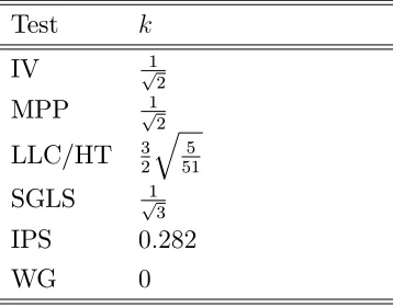
Table 1 compares the long T version of the IV test with the tests found in Moon et al. (2007), Moon and Perron (2008) and Harris et al. (2010), assuming homogeneous alternatives i.e. ci =cand thus E(ci) = c. The IV test has the maximum possible power which is equal

to that of the common point-optimal test of Moon et al. (2007). The large T version of the Harris and Tzavalis (1999) test coincides with the LLC test as can be seen from Madsen (2010). The WG test has trivial power in this case.

Table 1: Slopes for large T tests. Test k

IV _p1 2

MPP _p1 2

LLC/HT 3 2

q 5 51

SGLS _p1 3

IPS 0:282

WG 0

3.2

Incidental trends

WG* panel unit root test: Kruiniger and Tzavalis (2002) propose a version of the WG test that allows for incidental trends. Consider an augmented annihilator matrixQ =

IT X(X0X) 1X0 whereX = [e; ]:MultiplyingM2withQ wipes o¤ both individual e¤ects

and incidental trends. A new problem in this case is that under the null, the covariance matrix estimator ^ is no longer consistent:

yi = ie+ui; i= 1; :::; N:

leading to

1

N

N

X

i=1

yi yi0 ! +E( 2i)ee0:

To remove the nuisance parameters a selection matrix (algebraically equivalent to the original selection matrix of Kruiniger and Tzavalis (2002)) is applied. De…ne the matrix M with elements mts = 0 if ts 6= 0 and mts = 1 if ts = 0: Then,tr(M ) = 0 and thus

1

tr(M ee0_)N

N

X

i=1

y0

iM yi !E( 2i): (23)

Result (23) means that the selection matrix W G

p = p;W G

tr( 0_{Q M)}

e0_{M e} M where p;W G is

a (T XT) matrix having in diagonals _f p; ::;0; :::p_g the corresponding elements of matrix

0_{Q and zero everywhere else, has the propertytr(} W G

estimator

tr( W G_p ^)_!tr( 0_{Q ) (24)}

Theorem 3 For model M2 under Condition 1, the assumption that the order of serial

cor-relation is at most p and as N _{! 1}:

p

NV^

1 2

W G ^ (^'W G 1

^

b

^ )!N( ckW G;1) as N !+1: (25)

where

kW G =

tr( 0_{Q ) +tr(F}0_{Q ) tr(} W G

p ) tr( 0 W Gp )

2tr((A_{W G} )2₎ ; (26)

^

'_{W G}= (

N

X

i=1

y0

i 1Q yi 1) 1(

N

X

i=1

y0

i 1Q yi);

^ b

^ =

tr( W G

p ^) 1

N

PN

i=1yi;0 1Q yi; 1 andAW G=

1

2( 0Q +Q W G

p W Gp 0). The proof is given in the appendix.

FOD panel unit root test: Breitung (2000) proposed an unbiased panel unit root test for

M2based on an appropriate transformation of the dependent and the independent variables. Moon et al. (2006) show analytically that its local power is zero at the natural rate of

T 1_N 1=2 _{and thus, that the incidental trends problem applies in this case as well. A}

…xed-T version of the test is proposed on the assumption that unbiasedness provides better power performance. The estimator '^_{F OD} equals that of Breitung (2000) plus 1. The dependent variable is transformed with the Helmert or forward orthogonal deviation transformation and thus the name of the test. The method is as follows: In a …rst step subtract the initial observations from all series as in the panel IV test of DWHT. Then, by multiplying zi with

matrix A and zi with matrix B:

E(z0

iB0A zi) = 0; (27)

where A and B are(T 1)XT de…ned as

A= 01XT

E

!

and B = 01X(T 2) 0 0

IT 2 0(T 2)X1 _T1 T 2 ! where E = 0 B B B B B B @ q T 2

T 1 0

q

T 3

T 2

. ..

0 q1₂

1 C C C C C C A , = 0 B B B B B B B B B B @ 1 1 T 1 1 T 1

0 1 1

T 2

1

T 2

... . .. ... ... . .. ... ... 1 1₂ 1₂

0 0 1 1

whereE is (T 2)X(T 1); is (T 1)XT and T 2 = 0

B B B B @

1 2

.. .

T 2

1

C C C C A

. Based on the above,

de…ne the FOD estimator as

^

F OD = 1 + N

X

i=1

z0

iB0A zi

N

X

i=1

z0

iB0Bzi

: (28)

The following theorem derives its asymptotic distribution.

Theorem 4 For model M2 under Condition 1, the assumption that the order of serial

cor-relation is at most p and as N _{! 1}:

p

NV^

1 2

F OD^F OD(^'F OD 1

^_{bF OD}

^_{F OD})!N( ckF OD;1) ; (29)

where

kF OD =

tr( 0_B0_{A ) +tr(B}0_{A ) +tr(} 0_B0_{A ) +tr(F}0_B0_{A ) tr(} 0 F OD

p ) tr( F ODp )

2tr((AF OD )2)

:

(30)

and ^b

^ =

tr( F OD

p ^) 1

N

PN

i=1z0iB0Bzi

, F OD

p = p;F OD tr_e(0_{M e}M)M where p;F OD is a (T XT) matrix having

in diagonals _f p; ::;0; :::p_g the corresponding elements of matrix and zero everywhere

else. = 0_B0_A+B0_{A: The variance is given by V}

F OD = 2tr((AF OD )2) where AF OD = 1

2( + 0

F OD

p F ODp 0). The proof is given in the appendix.

The FOD test is unbiased when there is no serial correlation, as in the large T case, but is no longer unbiased when there is. It is then corrected for its bias in a similar way with the WG* test. The mean value in (27) applies only if V ar(ui) = 2IT and thus, so does

consistency. This can be seen in

p lim

N!1(^F OD 1) = tr( ) (31)

where tr( ) = 0 if and only if = 2_I

T:

IV test to allow for incidental trends. Take …rst di¤erences in model M2 :

yi =' yi 1+ (1 ') ie + ui; i= 1; :::; N: (32)

where yi = (yi2; :::; yiT)0; yi 1 = (yi1; :::; yiT 1)0; yi 2 = (yi0; :::; yiT 2)0;ui = (ui2; :::; uiT)0;

ui 1 = (ui1; :::; uiT 1)0 ande = (1;1; :::;1)are(T 1)X1vectors. From these series subtract

the initial observation yi1 to …nd

y_i ='y_{i 1}+ (1 ')a_i +u_i; i= 1; :::; N: (33)

where y_i = yi yi1e; yi 1 = yi 1 yi1e and ai = ( i yi1):Model (33) clearly

shows that moments similar to (7) can be exploited to test the null hypothesis of a unit root.Speci…cally:

E(y 0

i 1 pui) = 0 (34)

where _p is a(T 1)X(T 1)matrix with unities in itsp+ 1diagonal and zeros everywhere else.

Theorem 5 For model M2 under Condition 1, the assumption that the order of serial

cor-relation is at most p and as N _{! 1}:

p

N(^'_IV 1) ^V_{IV !}N( ck_IV;1) (35)

where

kIV =

tr( 0

p )

p

2tr((A_IV )2₎ (36)

and '^_IV = (

N

X

i=1

y 0

i 1 pyi 1) 1(

N

X

i=1

y 0

i 1 pyi); V =

2tr((AIV ) 2

)

tr( 0

p )2; AIV =

1

2( 0 p + p0 ):

is a (T 1)X(T 1) version of and = 2 1 2 02 where 1 = E(uiu0i) and

2 =E(uiu0i 1). The proof is given in the appendix.

The incidental trends problem appears to be relevant in the …xed-T literature as the WG* and FOD tests have trivial local power when there is no serial correlation. However, serial correlation, depending on its form, provides evidence in favour of the null or the alternative hypothesis which results in tests with non-trivial power or a bias. The DDIV test is superior to the WG* and FOD tests since it has power even when there is no serial correlation.

estimator is bias corrected for both its numerator and its denominator. The WG* and FOD tests are bias corrected only for their numerator therefore other versions of these tests that correct for both the numerator and the denominator might be more powerful. This motivates the following proposition:

Proposition 1 For model M2 under Assumptions 1, 2, the assumption that the order of serial correlation is zero and as N _{! 1}:

a) pNV^

1 2

HT '^W G 1

tr( 0_{Q )}

tr( 0_{Q )} ! N(0;1) ,

b) pN V

1 2

F OD(^F OD 1) ! N(0;1) ,

where VHT = 15(193T

2

728T+1147)

112(T+2)3_{(T 2)} and V_{F OD} =

2tr((A )2

)

tr(( 0_+IT)B0_{B( +IT))}2: A proof is given in the

appendix.

The previous theorem derives the asymptotic local power of the WG* and FOD based tests having both their numerators and denominators bias corrected. This case cannot accommodate serial correlation in the way that the WG* and the FOD tests did because the method would result in an identity. Both tests have trivial local power and can be thought of as part of the incidental parameters problem. Result a) is …rst found by Harris and Tzavalis (1999). For an intercept only case see e.g. Madsen (2010).

4

Assuming MA(1) serial correlation

The results of the above section are very general to provide some intuition about the behav-iour of tests. This section studies focuses on the simple and representative case of MA(1) errors.

Assumption 3: _fuitg is generated as uit = vit + vit 1 with 6= 1 and vit

N IID(0; 2 u):

4.1

Individual intercepts

The following two corollaries provide simpli…ed results for the IV and WG tests.

Corollary 2 Under assumptions 1,2 and 3, kIV depends only on T; p and : For selected cases of p and ; kIV(p; ) is given by:

kIV(0;0) =

r

1 2(T

kIV(1;0) =

r

T2

2 3T

2 + 1; (38)

kIV(2;0) =

r

T2

2 5T

2 + 3; (39)

kIV(3;0) =

r

T2

2 7T

2 + 6; (40)

kIV(1; ) =

D1;IV 2+D2;IV +D1;IV

q

R1;IV 4+R2;IV 3+R3;IV 2+R2;IV +R1;IV

; (41)

where Di;IV and Rj;IV for i = 1;2 j = 1;2;3; are functions of T and are given in the

appendix. The dependence of kIV on T is evident and thus supressed.

Relation (37) is the slope parameter of the original Breitung and Meyer (1994) test, found also by Bond et al. (2005) and Madsen (2010). Relations (41) and (38) coincide with those found by De Wachter, Harris and Tzavalis (2007).

Corollary 3 Under assumptions 1,2 and 3, kW G depends only onT; p and so for selected cases of p and ; kW G(p; ) is given by:

kW G(0;0) =

p

3(T 1)

q

T2 _2T 4

T + 5

; (42)

kW G(1;0) =

p

3(T2 _{3T + 2)}

TqT2 _6T 24

T +

12

T2 + 17

; (43)

kW G(2;0) =

p

3(T2 _{5T + 6)}

TqT2 _10T 80

T +

60

T2 + 41

; (44)

kW G(3;0) =

p

3(T2 _{7T + 12)}

TqT2 _14T 196

T +

192

T2 + 77

; (45)

kW G(1; ) =

(T 2)(T 2 2+ 3T 7 +T 1)

2T

q

R1;W G 4+R2;W G 3+R3;W G 2+R2;W G +R1;W G

; (46)

where R1;W G; R2;W G and R3;W G are functions of T de…ned in the appendix.

means that for = 0 there is one more moment available.

because the bias correction a¤ects the slope throughtr( p;W Gt ) +tr( 0 p;W G ):Since it

is subtracted, large negative values increase the slope and thus the power of the test. For

< 0 it takes positive values and thus reduces the power of the test. As T increases this e¤ect becomes stronger. For > 0; tr( p;W Gt ) +tr( 0 p;W G ) it is negative and thus

moves the limiting distribution towards the critical region.

4.2

Individual trends

The following corolaries correspond to the tests WG*, FOD and DDIV. Complexity of the slope parameteres makes analytical formulas unavailable for the cases of WG* and FOD*.

Corollary 4 Under assumptions 1,2 and 3 the following result holds:

k_{W G}(p;0) = 0 for p= 0;1;2; :::; T 2: (47)

k_{W G}(1; ) ₆= 0 for ₆= 0 (48)

A proof is given in the appendix.

Corollary 5 Under assumptions 1,2 and 3 the following result holds:

kF OD(p;0) = 0 for p= 0;1;2; :::; T 2: (49)

kF OD(1; ) 6= 0 for 6= 0 (50)

A proof is given in the appendix.

Corollary 6 Under assumptions 1,2 and 3, k_IV depends only onT; p and so for selected cases of p and ; kIV(p; ) is given by:

kDDIV(p;0) =

T p 3

p

2(T p 2) (51)

kDDIV(1; ) =

(T 4) 2 +T 4

q

2(P1 4+P2 3+P3 2+P2 +P1)

(52)

where polynomials P1; P2; and P3 are given in the appendix. A proof is given also in the appendix.

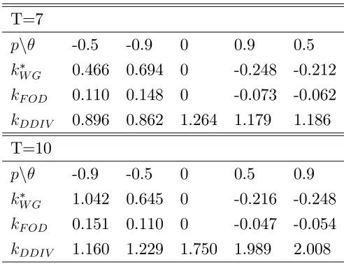
Table 2: Slope parameter values. T=7

p_n -0.5 -0.9 0 0.9 0.5

k_{W G} 0.466 0.694 0 -0.248 -0.212

kF OD 0.110 0.148 0 -0.073 -0.062

kDDIV 0.896 0.862 1.264 1.179 1.186

T=10

p_n -0.9 -0.5 0 0.5 0.9

k_{W G} 1.042 0.645 0 -0.216 -0.248

kF OD 0.151 0.110 0 -0.047 -0.054

kDDIV 1.160 1.229 1.750 1.989 2.008

Table 2 contains values of the slope parameters for the WG*, FOD and DDIV tests. The "incidental trends" problem is evident for = 0:Negative values of the moving average parameter result in non-trivial power while positive result in bias for tests WG* and FOD and the opposite for the DDIV test. This means that serial correlation a¤ects power in the opposite way than it did for tests that had only individual intercepts, except for the DDIV test.

It is easy to see that forT _{! 1}; k_IV = T p 3

Tp2(T p 2) !0;thus, in a largeT;the incidental

parameter problem remains. This is already known as Moon et al. (2007) derive the local power envelope for this case.

5

Simulation Results

This section presents some Monte Carlo results whose purpose is to show how good the asymptotic theory approximates the small sample results. Every experiment is conducted 5000 times. T=7 forM1and 15 for M2. All nuisance parameters that do not appear in the above local power functions are a priori set to zero, such as: ai = 0; i = 0; yi0 = 0:The local

alternatives are set as ' = 1 c=pN for N _{2 f}50;100;200;300;1000_g and c_{2 f}0;1_g: The errors are generated according to assumption 3 with _{2 f} 0:5;0;0:5_gandvit N IID(0;1):

The size is selected to be 0.05.

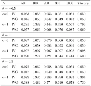
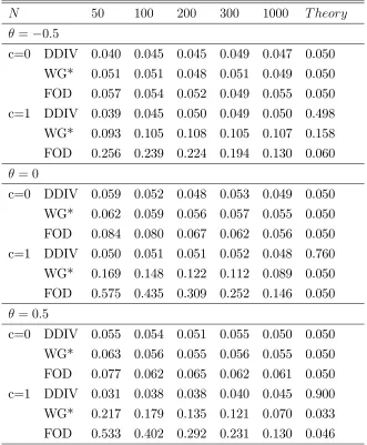
Table 3 shows that for M1 the approximation is very good, especially for the IV test. Both size and power are close to their theoretical values. Table 4 shows that for modelM2

test converges from above. The DDIV has size close to the nominal but also local power close to the size of the test, the approximation in this case is very poor.

Table 3: Size and local power for the IV and WG tests.

N 50 100 200 300 1000 T heory

= 0:5

c=0 IV 0.053 0.053 0.053 0.051 0.051 0.050 WG 0.045 0.050 0.047 0.049 0.043 0.050 c=1 IV 0.285 0.382 0.444 0.496 0.567 0.793 WG 0.057 0.066 0.068 0.076 0.087 0.069

= 0

c=0 IV 0.087 0.073 0.070 0.066 0.066 0.050 WG 0.058 0.058 0.053 0.053 0.049 0.050 c=1 IV 0.997 0.997 0.997 0.997 0.998 0.998 WG 0.220 0.274 0.321 0.344 0.414 0.500

= 0:5

c=0 IV 0.072 0.062 0.058 0.055 0.054 0.050 WG 0.047 0.049 0.049 0.048 0.052 0.050 c=1 IV 0.979 0.985 0.988 0.990 0.993 0.994 WG 0.388 0.489 0.57 0.610 0.678 0.730

6

Conclusions

This paper examines the power properties of …xed-T tests under serial correlation. Two models are considered, one that has individual intercepts and one that has both individual intercepts and incidental trends. For the …rst model, asymptotic local power functions of the WG and the IV test show that the two tests behave di¤erently but the IV test is superior to the WG test in many aspects. In the context of MA(1) errors the IV test is always more powerful than the WG. Furthermore, its power increases with T irrespective of the moving average parameter and it is never biased. The WG test shows great gains or losses of power that depend on the sign of the moving average parameter. For both tests positive values support greater power while negative values lead to power loss. This loss can even result in bias for the WG test.

like the IV test but has less power.

Table 4:Size and local power for tests WG*, FOD and DDIV.

N 50 100 200 300 1000 T heory

= 0:5

c=0 DDIV 0.040 0.045 0.045 0.049 0.047 0.050 WG* 0.051 0.051 0.048 0.051 0.049 0.050 FOD 0.057 0.054 0.052 0.049 0.055 0.050 c=1 DDIV 0.039 0.045 0.050 0.049 0.050 0.498 WG* 0.093 0.105 0.108 0.105 0.107 0.158 FOD 0.256 0.239 0.224 0.194 0.130 0.060

= 0

c=0 DDIV 0.059 0.052 0.048 0.053 0.049 0.050 WG* 0.062 0.059 0.056 0.057 0.055 0.050 FOD 0.084 0.080 0.067 0.062 0.056 0.050 c=1 DDIV 0.050 0.051 0.051 0.052 0.048 0.760 WG* 0.169 0.148 0.122 0.112 0.089 0.050 FOD 0.575 0.435 0.309 0.252 0.146 0.050

= 0:5

c=0 DDIV 0.055 0.054 0.051 0.055 0.050 0.050 WG* 0.063 0.056 0.055 0.056 0.055 0.050 FOD 0.077 0.062 0.065 0.062 0.061 0.050 c=1 DDIV 0.031 0.038 0.038 0.040 0.045 0.900 WG* 0.217 0.179 0.135 0.121 0.070 0.033 FOD 0.533 0.402 0.292 0.231 0.130 0.046

As a by-product of the above analysis, the problem …rst encountered by Moon and Phillips (1999) and named "incidental trends" is discussed. Asymptotic local power is found only when there is serial correlation for the WG* and FOD tests and always for the DDIV test.

References

[1] Bond, S., Nauges, C., and Windmeijer, F., 2002. Unit roots: Identi…cation and testing in micropanels. Cemmap Working Paper CWP07/05, The Institute for Fiscal Studies, UCL.

[2] Breitung J., 2000. The local power of some unit root tests for panel data. In Badi H. Baltagi, Thomas B. Fomby, R. Carter Hill (ed.) Nonstationary Panels, Panel Cointe-gration, and Dynamic Panels (Advances in Econometrics, Volume 15), Emerald Group Publishing Limited, pp.161-177.

[3] Breitung J., Meyer W., 1994. Testing for unit roots using panel data: are wages on di¤erent bargaining levels cointegrated? Applied Economics 26, 353-361.

[4] De Blander, R., Dhaene, G., 2011. Unit Root Tests for Panel Data with AR(1) Errors and Small T. Econometrics Journal. 15(1), 101-124.

[5] De Wachter, S., Harris, R.D.F., Tzavalis, E., 2007. Panel unit root tests: the role of time dimension and serial correlation. Journal of Statistical Inference and Planning, 137, 230-244.

[6] Hahn, J., Kuersteiner, G., 2002. Asymptotically unbiased inference for a dynamic panel model with …xed e¤ects when both n and T are large. Econometrica. 70, 1639-1657.

[7] Han C., & Phillips, Peter C. B., 2010. Gmm Estimation For Dynamic Panels With Fixed E¤ects And Strong Instruments At Unity. Econometric Theory, Cambridge University Press, vol. 26(01), pages 119-151.

[8] Harris, R.D.F., Tzavalis, E., 1999. Inference for unit roots in dynamic panels where the time dimension is …xed. Journal of Econometrics. 91, 201-226.

[9] Harris, R.D.F., Tzavalis, E., 2004. Inference for unit roots for dynamic panels in the presence of deterministic trends: Do stock prices and dividends follow a random walk ?. Econometric Reviews. 23, 149-166.

[10] Hayakawa K., 2010. A unit root test for micro panels with serially correlated errors. Working Paper, Hiroshima University.

[12] Kruiniger, H., and E., Tzavalis, 2002. Testing for unit roots in short dynamic panels with serially correlated and heteroscedastic disturbance terms. Working Papers 459, Department of Economics, Queen Mary, University of London, London.

[13] Levin, A., Lin, F., and Chu, C., 2002. Unit root tests in panel data: asymptotic and …nite-sample properties. Journal of Econometrics 122, 81–126.

[14] Madsen E. 2010. Unit root inference in panel data models where the time-series dimen-sion is …xed: a comparison of di¤erent tests. Econometrics Journal, 13, 63-94.

[15] Moon, H.R. & B. Perron (2004) Asymptotic Local Power of Pooled t-Ratio Tests for Unit Roots in Panels with Fixed E¤ects. Mimeo, University of Southern California.

[16] Moon, H. R. and B. Perron (2004). Testing for a unit root in panels with dynamic factors. Journal of Econometrics 122, 81–126.

[17] Moon, H. R., B. Perron and P. C. B. Phillips (2006). A note on “The local power of some unit root tests for panel data” by Breitung. Econometric Theory 22, 1177–88.

[18] Moon H.R., Perron B. & Phillips P.C.B., 2007. Incidental trends and the power of panel unit root tests. Journal of Econometrics, 141(2), 416-459.

[19] Moon H.R., and Perron B., 2008. Asymptotic local power of pooled t-ratio tests for unit roots in panels with …xed e¤ects. Econometrics Journal, 11, 80-104.

[20] Moon H.R., and P. C. B. Phillips (1999). Maximum Likelihood Estimation in Pan-els with Incidental Trends. Oxford Bulletin of Economics and Statistics, Special Issue (1999), 0305-9049.

[21] Sargan, J. D. and A. Bhargava (1983). Testing residuals from least squares regression for being generated by the Gaussian random walk. Econometrica 51, 153–74.

[22] Schwert, G.W., 1989. Tests for unit roots:a Monte Carlo investigation. Journal of Busi-ness and Economic Statistics 7, 147–160.

7

Appendix

Proof of Theorem 1 Under local alternatives the statistic is written as:

p

N(^'_IV '_N) = pN

0

B B B B @ 1 N

N

X

i=1

z0

i 1 pui+_N1

N

X

i=1

(1 'N)aizi0 1 pe

1 N

N

X

i=1

z0

i 1 pzi 1

+'_N '_N

1

C C C C A

=

=

1

p

N N

X

i=1

z0

i 1 pui+p1_N

N

X

i=1

(1 '_N)aiz0i 1 pe

1 N

N

X

i=1

z0

i 1 pzi 1

= (A) + (B)

(C) (53)

Under the alternative:

y 1 =wyi0+ e(1 'N)ai+ ui; i= 1; :::; N: (54)

where

=

0

B B B B B B B B B B B @

0 : : : : : 0

1 0 :

'_N 1 : :

'2

N 'N : : :

: : : : :

: : 1 0 :

'T_N 2 'T_N 3 : : '_N 1 0

1

C C C C C C C C C C C A

(55)

and w= (1; '_N; '2

N; :::; 'TN 1)0: For'N = 1: : The …rst order Taylor expansions of

and w are:

= +F('_N 1) +op(1) and (56)

w = e+f('_N 1) +oP(1) (57)

where F = _d'd

N j'N=1 and f =

dw

d'N j'N=1 : Then,

zi 1 =yi 1 eyi0 = (w e)yi0+ e(1 'N)ai+ ui (58)

1

p

N N

X

i=1

z0

i 1 pui = p1_N

N

X

i=1

((w e)yi0 + e(1 'N)ai + ui)0 pui = p1_N N

X

i=1

yi0(w

e)0

pui + (1 'N)aie0 0 pui+ui 0 pui:

But

1

p

N

N

X

i=1

yi0(w e)0 pui p

!0 (59)

1

p

N

N

X

i=1

(1 'N)aie0 0 pui p

!0 (60)

1

p

N

N

X

i=1

ui 0 pui d

!N(0; VIV;1) (61)

because by construction of p : tr( 0 p ) = tr(F0 p ) = 0: The previous limits occur

after substituting (56) and (57) and by using standard results on quadratic forms found in Schott (1997). Also (B) and (C) :

1

p

N

N

X

i=1

(1 '_N)aiz0i 1 pe p

!0 (62)

1

N

N

X

i=1

z0

i 1 pzi 1

p

!tr( 0

p ) (63)

Combining (53)-(63)

p

N(^'IV 'N) d

!N(0; VIV;1

tr( 0 _{p )}2) (64)

p

N(^'_IV 1) d_!N( c; VIV)

p

N(^'IV 1)V 1=2 IV

d

!N( pc

VIV

;1) (65)

Proof of Theorem 2 The proof is segmented in two parts. Part A contains proof forc= 0

that can be directly compared to that of Kruiniger and Tzavalis (2002), Part B contains the proof for c >0.

A) To derive the limiting distribution of the test statistic of the theorem, we will proceed into stages. We …rst show that the LSDV estimator'^W G is inconsistent, asN ! 1. Then,

will construct a normalized statistic based on'^W G corrected for its inconsistency (bias) and

derive its limiting distribution under the null hypothesis of' = 1, asN _{! 1}. Decompose the vector yi; 1 for model (1) under hypothesis ' = 1 as

where the matrix is is a (T XT) matrix de…ned as r;c = 1, if r > cand 0 otherwise.

Premultiplying (66) with matrix Qyields

Qyi; 1 =Q ui, (67)

since Qe= (0;0; :::;0)0_{. Substituting (67) into '^}

W G :

^

'_{W G} 1 =

1 N

PN

i=1yi;0 1Qui

1 N

PN

i=1yi;0 1Qyi; 1

=

1 N

PN

i=1u0i 0Qui

1 N

PN

i=1u0i 0Q ui

. (68)

By Kitchin’s Weak Law of Large Numbers (KWLLN), we have

1 N N X i=1 u0

i 0Qui

p

!tr( 0_{Q ) and} 1

N

N

X

i=1

u0

i 0Q ui

p

!tr( 0_{Q ), (69)}

where " _!p " signi…es convergence in probability. Using the last results, the yet non stan-dardized statistic can be written by (68) as

p

N^ '^_{W G} 1 ^b ^

!

= pN^

1 N

PN

i=1y0i; 1Qui

^

tr( p;W G^)

^

!

= pN 1 N

N

X

i=1

y0

i; 1Qui

1 N N X i=1 y0

i p;W G yi

!

. (70)

where

^ = 1

N

N

X

i=1

y0

i p;W G yi (71)

Since, under the null hypothesis = 1, we haveui = yi, the last relationship can be written

as follows:

p

N '^_{W G} 1 ^b ^

!

= pN 1 N

N

X

i=1

u0

i 0Qui

1 N N X i=1 u0

i p;W Gui

!

= p1

N

N

X

i=1

u0

i( 0Q p;W G)ui =

1 p N N X i=1

tr[( 0_Q

p;W G)uiu0i] (72)

= p1

N

N

X

i=1

where Wi constitute random variables with mean

E(Wi) = E[u0i( 0Q p;W G)ui] =tr[( 0Q p;W G)E(uiu0i)]

= tr( 0_Q

p;W G) = 0, for alli,

since tr( 0_{Q) =tr(}

p;W G) (ortr( 0Q p;W G) = 0) and variance

V ar(Wi) =V ar(u0i( 0Q p;W G)ui) = 2tr((AW G )2): (73)

The results of Theorem 2 follow by applying Lindeberg-Levy central limit theorem (CLT) to the sequence of IID random variables Wi. The last relation follows from standard linear

algebra results (see e.g. Schott(1997).

B) The following proof applies forc >0. Also after subtracting yi 1 from both sides of

(1):

yi =ui+ ('N 1)yi 1+ (1 'N)aie (74)

In a …rst step we …nd the distribution of the unstandardized statistic around '_N :

^p_N(^'

W G ^ b

^ 'N) = ^

p

N('N +

1 N

N

X

i=1

y0 i 1Qui

1 N

N

X

i=1

y0 i 1Qy0i 1

^ b

^ 'N) =

p

N(_N1

N

X

i=1

y0

i 1Qui

tr( p;W G^) =

p

N(1 N

N

X

i=1

y0

i 1Qui _N1

N

X

i=1

y0

i p;W G yi) =

1

p

N

N

X

i=1

y0

i 1Qui

1

p

N

N

X

i=1

y0

i p;W G yi = (C) (D): (75)

We then apply the Lindeberg-Levy CLT to …nd the limiting distributions of (C) and (D):

For(C) :

1

p

N N

X

i=1

y0

i 1Qui = p1_N

N

X

i=1

(wyi0+ e(1 'N)ai+ ui)0Qui =

1

p

N

N

X

i=1

yi0w0Qui+ai(1 'N)e0 0Qui+u0i 0Qui (76)

To …nd the limit of (76) we …rst …nd every limit separately: In all quantities we substitute

w and with their Taylor expansions given in (56) and (57) respectively and we substitute

1 p N N X i=1

yi0w0Qui = p1_N N

X

i=1

yi0(e+f('N 1) +oP(1))0Qui =

1 p N N X i=1

yi0e0Qui+

1

N

N

X

i=1

f0_Qu

iyi0+op(1)

p

!0;because (77)

1

N

N

X

i=1

f0_Qu

iyi0 ! f0QE(uiyi0) = 0 by Assumption 2 and

1 p N N X i=1

yi0e0Qui = 0because e0Q= 0:

The second summand: _p1 N

N

X

i=1

ai(1 'N)e0 0Qui = _Nc N

X

i=1

aie0( 0+F0(p_Nc) +op(1))Qui =

c N

N

X

i=1

aie0 0 Qui

c2

N3=2 N

X

i=1

aie0F0Qui+op(1) p

!0 because (78)

c N

N

X

i=1

aie0 0 Qui ! cie0 0 QE(aiui) = 0; by Assumption 2 and

c2

N3=2 N

X

i=1

aie0F0Qui p

!0due to the fast rate that 1

N3=2 goes to zero.

Then the third summand: p1

N N

X

i=1

u0

i 0Qui = p1_N

N

X

i=1

u0

i( 0+F0(p_Nc ) +op(1))Qui =

= _p1

N

N

X

i=1

u0

i 0Qui

c N N X i=1 u0

iF0Qui+op(1) (79)

c N N X i=1 u0

iF0Qui ! ctr(F0Q ) (80)

p

N(1

N

N

X

i=1

u0

i 0Qui tr( 0Q ))

d

!N(0; VW G;1) (81)

The variance VW G;1 is known due to the normality assumption in Assumption 1 but we

to be subtracted, so that the limiting distribution is centered around 0: There is no reason to do so because later, relation (83) requires pN tr( p;W G ) to be subtracted. But by

construction, tr( 0_{Q ) = tr(}

p;W G ) and thus, cancel out. By adding the results of (77),

(78) and (79):

1 p N N X i=1 y0

i 1Qui

d

!N( ctr(F0_{Q ); V}

W G;1): (82)

The proof for the limiting distribution of (D) is more tedious but it follows the same steps: After substituting (74) in (D)

1 p N N X i=1 y0

i p;W G yi = p1_N

N

X

i=1

(ui+('N 1)yi 1+(1 'N)aie)0 p;W G(ui+('N 1)yi 1+

(1 '_N)aie) =

= _p1 N

N

X

i=1

u0

i p;W Gui+u0i p;W Gyi 1('N 1)+u0i p;W Ge(1 'N)ai+('N 1)y0i 1 p;W Gui+

('N 1)2y0i 1 p;W Gyi 1+ ('N 1)yi0 1 p;W Ge(1 'N)ai+

(1 'N)aie0 p;W Gui+ (1 'N)aie0 p;W Gyi 1('N 1) + (1 'N)2a2ie0 p;W Ge:

Then by the same arguments that gave (77), (78) and (79) we have:

p N 1 N N X i=1 u0

i p;W Gui

d

tr( p;W G )

!

d

!N(0; VW G;2) (83)

1 p N N X i=1 u0

i p;W Gyi 1('N 1)

p

! ctr( p;W G ) (84)

1 p N N X i=1 u0

i p;W Ge(1 'N)ai

p

!0 (85)

1 p N N X i=1

('_N 1)y0

i 1 p;W Gui

p

! ctr( 0

p;W G ) (86)

1 p N N X i=1

('N 1)2y0i 1 p;W Gyi 1

p

!0 (87)

1 p N N X i=1

('N 1)y0i 1 p;W Ge(1 'N)ai

p

!0 (88)

1 p N N X i=1

(1 'N)aie0 p;W Gui

p

!0 (89)

1 p N N X i=1

(1 '_N)aie0 p;W Gyi 1('N 1)

p

!0 (90)

1 p N N X i=1

(1 '_N)2a2_ie0

p;W Ge

p

Combining the results (83)-(91) we …nd that:

1

p

N

N

X

i=1

y0

i p;W G yi !N( ctr( 0 p;W G ) ctr( p;W G ); VW G;2) (92)

Thus from relations (82) and (92):

^p_N(^'

W G

^

b

^ 'N) d

!N( c(tr(F0_{Q ) tr(} 0

p;W G ) tr( p;W G )); VW G) (93)

Notice that VW G 6= VW G;1 +VW G;2 because (C) and (D) are correlated. VW G can be

easily calculated from the variances of (C) and (D) and the covariance between them but the result is straightforward when noticing that the quantities to which the CLT applies do not depend on c: Finally as before

1

N

N

X

i=1

y0

i 1Qyi 1

p

!tr( 0_{Q ) (94)}

Therefore the variance of the test is the same under the null and under local alternative hypotheses. Substituting (4) to (93):

^p_N(^'

W G

^_b ^ 1 +

c

p

N)

d

!N( c(tr(F0_{Q ) tr(}

p;W G ) tr( p;W G )); VW G)

^p_N(^'

W G

^_b ^ 1)

d

!N( c(tr( 0_{Q ) +tr(F}0_{Q ) tr(}

p;W G ) tr( p;W G )); VW G)

^p_N(^'

W G

^_b ^ 1)V

1=2 W G

d

!N( ctr(

0_{Q ) +tr(F}0_{Q ) tr(}

p;W G ) tr( p;W G )

p

VW G

;1):

(95)

Proof of Theorem 3 The main point of departure from the proof of theorem 2 is:

yi 1 =wyi0+ X i+ ui; i= 1; :::; N: (96)

where _i = (1 'N)ai+' i (1 'N) i

!

= (1 '_N) ai

i

!

+'_N i

0

!

= _pc N

ai i

i

!

+

i

1 0

!

= pc

N i+ ie wheree =

1 0

!

: Thus

i =

c

p

N i+ ie (97)

and

Following the same steps with the proof of theorem 2:

^ p_N(^'

KT ^ b

^ 'N) = p1_N N

X

i=1

y0

i 1Q ui p1_N

N

X

i=1

y0

i W Gp yi = (A ) (B ): Then

(A ) = p1

N N

X

i=1

y0

i 1Q ui = p1_N

N

X

i=1

(wyi0+ X i+ ui)0Q ui:

1 p N N X i=1

yi0w0Q ui ! 0 (99)

1 p N N X i=1 0

iX 0Q ui ! 0 (100)

1 p N N X i=1 u0

i Q ui ! N(tr( 0Q ) ctr(F0Q ); VKT;1) (101)

Limits in (99) and (101) are derived as before. To see why (100) stands:

1 p N N X i=1 0

iX 0Q ui = p1_N

N

X

i=1

(_pc

N i+ ie )

0_X 0_{Q u}

i = _Nc

N

X

i=1

0

iX 0Q ui+p1_N

N

X

i=1

ie 0X 0Q ui:

But c N N X i=1 0

iX 0Q ui ! 0 (102)

1 p N N X i=1

ie 0X 0Q ui =

1 p N N X i=1

ie 0X 0Q ui = 0; (103)

since e 0_X 0_{Q = (0; :::;0).}

(B ) = p1

N N

X

i=1

y0

i W Gp yi = p1_N

N

X

i=1

(ui+ ('N 1)yi 1+X i)0 W Gp (ui+ ('N 1)yi 1+

X _i) =

= p1

N N

X

i=1

u0

i W Gp ui +u0i W Gp yi 1('N 1) +ui0 W Gp X i + ('N 1)y0i 1 W Gp ui + ('N

1)2_y0

i 1 W Gp yi 1+ ('N 1)y0i 1 W Gp X i+

0

Then

1

p

N

N

X

i=1

u0

i W Gp ui ! N(tr( W Gp ); VKT;1) (104)

1

p

N

N

X

i=1

u0

i W Gp yi 1('N 1) ! ctr( W Gp ) (105)

1

p

N

N

X

i=1

u0

i W Gp X i ! 0 (106)

1

p

N

N

X

i=1

('N 1)yi0 1 W Gp ui ! ctr( 0 W Gp ) (107)

1

p

N

N

X

i=1

('N 1)2yi0 1 W Gp yi 1 ! 0 (108)

1

p

N

N

X

i=1

('N 1)yi0 1 W Gp X i ! cE( 2i)e 0X0 0 W Gp Xe (109)

1

p

N

N

X

i=1

0

iX0 W Gp ui ! 0 (110)

1

p

N

N

X

i=1

0

iX W Gp yi 1('N 1) ! cE( 2i)e 0X0 W Gp Xe (111)

1

p

N

N

X

i=1

0

iX W Gp X i ! ctr(X0 W Gp Xe E( 0i i)) +ctr(e 0X0 W Gp XE( i i(112)))

De…neE( _{i i}) =E( 2_i)~e where ~e = 1

1

!

Combining (104)-(112)

^ p_N(^'

KT

^_b

^ 1)!N( c(C+E(

2

i)D); VKT) (113)

wher

C = tr( 0_{Q ) +tr(F}0_{Q ) tr(} W G

p ) tr( 0 W Gp )and (114)

D = tr(X0 W G

p Xe e~0) +tr(e 0X0 W Gp X~e) e 0X0 0 W Gp Xe e 0X0 W Gp Xe (115)

To reach the …nal result the following identities hold:

tr(X0 W G

p Xe e~0) = e 0X0 0 W Gp Xe (116)

tr(e 0_X0 W G

Thus

^ p_N(^'

KT

^

b

^ 1)V

1=2

KT !N( c

tr( 0_{Q ) +tr(F}0_{Q ) tr(} W G

p ) tr( 0 W Gp )

p

V_KT ;1)

(118) As can be seen the nuisance parameters do not a¤ect the distribution.

Proof of Theorem 4 In the following derivations we use the following equations, under the null and the alternative:

zi = 'Nzi 1+X i+ui; (119)

zi 1 = X i+ ui+ (w e)yi0; (120)

zi = ('N 1)zi 1+X i+ui: (121)

We start by showing its asymptotic distribution under the null.

^

'_B 1 =

1 N N X i=1 z0

iB0A zi

1 N N X i=1 z0

iB0Bzi

= (A) (B)

Then (A) : 1 N

N

X

i=1

z0

iB0A zi = _N1

N

X

i=1

(z0

i 1+ ie0+ui0)B0A( _ie+u_i) = 1

N N

X

i=1

(u0

i 0+ ie0 0+

ie0+ui0)B0A( _ie+u_i) = _N1

N

X

i=1

(u0

i( 0+IT) + i 0)B0A( ie+ui) = _N1

N

X

i=1

u0

i( 0+IT)B0Aui

because ( +IT)e= ; 0B0 = 01XT and B0Ae= 0T X1:

1 N N X i=1 u0

i( 0+IT)B0Aui =

1 N N X i=1 u0

i ui !tr( ): (122)

since ( 0_+I

T)B0A= by de…nition. Thus iftr( ) = 0the test is unbiased. This happens

only if = 2_I

T;both homoscedasticity and non-autocorrelation are essential.

(B) : _N1

N

X

i=1

z0

iB0Bzi = _N1

N

X

i=1

(z0

i 1+ ie0+ui0)B0B(z_{i 1}+ _ie+u_i) = _N1

N

X

i=1

(u0

i( 0+IT) +

i 0)B0B(( +IT)ui+ i ) = N1

N

X

i=1

u0

i( 0+IT)B0B( +IT)ui and thus

1 N N X i=1 u0

Result (123) is only used in the no serial correlation version of the FOD test. The proof of this version is straightforward along the lines of the proof of theorem 2. The rest of this proof is focused on the general form of the FOD test. The test statistic

p

N^F OD(^'F OD 1

^

bF OD

^_{F OD}) =

p

N 1 N

N

X

i=1

z0

iB0Bzi

! 0

B B B B @

1 +

1 N

N

X

i=1

z0

iB0A zi

1 N

N

X

i=1

z0

iB0Bzi

1

1 N

N

X

i=1

z0

i F ODp zi

1 N

N

X

i=1

z0

iB0Bzi

= pN 1 N

N

X

i=1

u0

i( 0+IT)B0Aui

1

N

N

X

i=1

z0

i F ODp zi

!

= pN 1 N

N

X

i=1

z0

i ( 0 +IT)B0A F ODp zi

!

= p1

N

N

X

i=1

z0

i F ODp zi (12

because z0

i( 0 +IT)B0A zi = ( ie0+u0i)( 0+IT)B0A( ie+ui) = ui0( 0+IT)B0Aui from

the identities above. Asymptotically, based on standard matrix algebra results:

1

p

N

N

X

i=1

z0

i F ODp zi !N(0;2tr(A2F OD)): (125)

The above concludes the proof for the distribution under the null. Under local alternatives, the proof follows the steps of the proof of theorem 3, notting that the following identities apply:

tr( ) = 0and tr( 0_B0_{A) = tr(B}0_A)

e0 _{= 0}

1XT and e= 0T X1

B0_{AXe~ = 0}

T X1

e 0_X0 0_B0_{A Xe = e} 0_X0 0_B0_AXe~

e 0_X0_B0_{A Xe = e} 0_X0_B0_AXe~

e 0_X0 F OD

p Xe = e 0X0 F ODp Xe~

e 0_X0 0 F OD

Proof of Theorem 5 Like the proof of Theorem 1. Under local alternatives

p

N(^'_IV '_N) = pN

0

B B B B @

N

X

i=1

y 0

i 1 pyi

N

X

i=1

y 0

i 1 pyi 1

'_N

1

C C C C A

= pN

0

B B B B @

N

X

i=1

y 0

i 1 p('Nyi 1+ (1 'N) ie +ui)

N

X

i=1

y 0

i 1 pyi 1

'_N

1

C C C C A

=

1

p

N N

X

i=1

(1 '_N) _iy 0

i 1 pe + p1_N

N

X

i=1

y 0

i 1 pui

1 N

N

X

i=1

y 0

i 1 pyi 1

:

Where

1

p

N

N

X

i=1

(1 '_N) _iy 0

i 1 pe ! 0;

1

p

N

N

X

i=1

y 0

i 1 pui ! N(0;2tr((AIV )2);

1

N

N

X

i=1

y 0

i 1 pyi 1 ! tr( 0 p );

since tr( 0

p ) = 0:

Proof of Proposition 1 This proof is more general than that of Madsen (2010). The latter can be seen as a special case of this by substitutingQ with Q:Under local alternatives the Harris and Tzavalis 1999 statistic can be written as

p

because, under the null, plim(^'_{W G} 1) = _trtr₍(00_QQ )₎:Then

p

N '^_{W G} 'N

tr( 0_{Q )}

tr( 0_{Q )} = p N 0 B B B B @ 1 N N X i=1 y0

i 1Q ('Nyi 1+X i+ui)

1 N N X i=1 y0

i 1Q yi 1

'N

tr( 0_{Q )}

tr( 0_{Q )}

1 N N X i=1 y0

i 1Q

1 N N X i=1 y0

i 1Q yi

= 1 p N N X i=1 y0

i 1Qui tr(

0_{Q )}

tr( 0_{Q )}y0i 1Q yi 1

! 1 N N X i=1 y0

i 1Q yi 1

= 1 p N N X i=1 y0

i 1Qui tr(

0_{Q )}

tr( 0_{Q )}

1 p N N X i=1 y0

i 1Q yi 1

1 N N X i=1 y0

i 1Q yi 1

Using similar arguments with the previous proofs and taking into account the fact that

tr( 0_{Q F)} tr( 0Q )

tr( 0_{Q )} +tr(F

0_{Q )} tr( 0Q )

tr( 0_{Q )} tr(tr(

0_{Q ) tr(F}0_{Q ) = 0 (127)}

leads to the result.

Proof of Corollary 1 The proof is straightforward from (9) and the results of Corollaries 3 and 4. As in De Wachter at al. (2007), scale the statistic withT and apply the continuous mapping theorem. The joint convergence is guaranteed by Hahn and Kuersteiner (2002) and De Wachter at al. (2007). However this proof, is not intuitive with regard to the local alternatives in this case. To clearly show that the largeT version of the test has a limiting distribution on the local alternatives'N T = 1 _Tpc_N we provide the following proof only for

the IV test. Consider,

^

'_IV =

N

X

i=1

T p 1

X

t=1

zitzit+p+1

N

X

i=1

T p_X1

t=1

zitzit+p

Then, under the above local alternatives

TpN(^'IV 'N T) = T

p

N

0

B B B B B @

N

X

i=1

T p_X1

t=1

zit('N Tzit+p+uit+p+1+ (1 'N T)ai)

N

X

i=1

T p 1

X

t=1

zitzit+p

'N T

1

C C C C C A

=

1

p

N 1 T

N

X

i=1

T p 1

X

t=1

(zituit+p+1+zit(1 'N T)ai))

1 N

1 T2

N

X

i=1

T p_X1

t=1

zitzit+p

: (129)

Notice that under local alternatives

zit = 'tN Tzi0+'N Tt 1uit 1+:::+uit (130)

= 't_{N T}1ui1+'N Tt 2ui2+:::+uit: (131)

Also, from the binomial theorem

't_{N T} = 1 +o(T): (132)

Inserting (132) in (130) we take

zituit+p+1 =ui1+:::+uit+o(T): (133)

The last equality allows the use of standard asymptotic results about AR(1) processes (see also Hamilton (1994)). To …nd the limiting distribution in (129) we show where the three sums converge:

1

p

N

1

T

N

X

i=1

T p 1

X

t=1

zit(1 'N T)ai =

1

p

N

N

X

i=1

ai

1

T

T p 1

X

t=1

zit

c TpN

= 1

N

N

X

i=1

ai

1

T2

T p_X1

t=1

zit:

Taking …rst T _{! 1};

1

T2

T p 1

X

t=1

and thus 1 p N 1 T N X i=1

T p 1

X

t=1

zit(1 'N T)ai !0: (134)

1 p N 1 T N X i=1

T p 1

X

t=1

zituit+p+1 =

1 p N N X i=1 1 T

T p 1

X

t=1

zituit+p+1: (135)

As T _{! 1};

1

T

T p_X1

t=1

zituit+p+1 !

1 2

2 _[W

i(1)]2 1 (136)

where W(r) denotes the standard Wiener process at time r: [Wi(1)]2 follows a chi-squared

distribution with one degree of freedom, thus, E_f[Wi(1)]2g = 1 and V arf[Wi(1)]2g = 2:

Then asN _{! 1} (135) becomes:

1 p N N X i=1 1 2

2 _[W

i(1)]2 1 !N(0;

4

2 ) (137)

Finally, the limit of the denominator comes from:

1 N 1 T2 N X i=1

T p 1

X

t=1

zitzit+p =

1 N N X i=1 1 T2

T p 1

X

t=1

zitzit+p (138)

Then

zit+p ='pN Tzit+ p

X

k=1

'k_{N T}1(1 '_{N T})ai+ p

X

k=1

'k_{N T}1uit+(p k 1) (139a)

Plugging (139a) into (138) and acknowledging (132):

1

T2

T p 1

X

t=1

'p_{N T}z_it2 = 1

T2

T p 1

X

t=1

z2_it+o(T)_! 2

1 Z

0

[Wi(r)]2dr (140)

1

T2

T p 1

X t=1 zit p X k=1

'k_{N T}1(1 'N T)ai ! 0 (141)

1

T2

T p 1

X t=1 zit p X k=1

'k_{N T}1uit+(p k 1) =

1

T2

T p 1

X t=1 zit p X k=1

uit+(p k 1)+o(T)!0 (142)

Inserting (140), (141) and (142) into (138) and asN _{! 1}:

1 N N X i=1 2 1 Z 0

[Wi(r)]2dr ! 2

2 (143)

Combining (134), (137) and (143)

TpN(^'_IV '_{N T}) _! N(0;2)

TpN(^'_IV 1) _! N( c;2):

Proof of Corollary 2 Assuming N = 2uIT an important identity is

2tr(AIV2) =tr( 0 p ); for eachp (144)

The following identities apply:

tr( 0

p ) =

1 2(T

2 _{T); for p= 0}

tr( 0

p ) =

[1₂(T 2)(T 1)]2 1

2T(T 3) + 1

; forp= 1

tr( 0

p ) =

T2

2 5T

2 + 3; for p= 2

tr( 0

p ) =

T2

2 7T

2 + 6; for p= 3 (145)

When a MA(1) process is assumed for the error term, De Wachter, Harris and Tzavalis (2007) …nd that:

D( ; T) = D1;IV 2 +D2;IV +D1;IV (146)

R( ; T) = R1;IV 4+R2;IV 3+R3;IV 2+R2;IV +R1;IV

where

D1;IV =

T2

2 3T

2 + 1

D2;IV = T2 4T + 4 (147)

R1;IV =

1

2T(T 3) + 1 (148)

R2;IV = 2T(T 5) + 12

R3;IV = 3T(T 5) + 20 (149)

Proof of Corollary 3 Substitute in (95) the following identities to derive the …nal results: