Optimal Multiperiodic Control for Inventory Coupled Systems: A Multifrequency Second Order Test

(1)

http://www.scirp.org/journal/ojop ISSN Online: 2325-7091

ISSN Print: 2325-7105

Optimal Multiperiodic Control for Inventory

Coupled Systems: A Multifrequency

Second-Order Test

Marek Skowron, Krystyn Stycze

ń

Department of Control Systems and Mechatronics, Wrocław University of Science and Technology, Wrocław, Poland

Abstract

A complex autonomous inventory coupled system is considered. It can take, for ex-ample, the form of a network of chemical or biochemical reactors, where the inven-tory interactions perform the recycling of by-products between the subsystems. Be-cause of the flexible subsystems interactions, each of them can be operated with their own periods utilizing advantageously their dynamic properties. A multifrequency second-order test generalizing the π_{-test for single systems is described. It can be}

used to decide which kind of the operation (the static one, the periodic one or the multiperiodic one) will intensify the productivity of a complex system. An illustrative example of the multiperiodic optimization of a complex chemical production system is presented.

Keywords

Optimal Multiperiodic Control, Complex Systems, Inventory Interactions, Nested Optimization, Multifrequency Second-Order Test

1. Introduction

We consider complex autonomous inventory coupled (IC) systems. Such systems can take, for example, the form of a network of chemical or biochemical networks, where the inventory interactions perform the recycling of by-products or by-streams from some subsystems to other subsystems as their input components or energy carriers [1]. Because of the flexible interactions of the subsystems, each of them can be operated with their own period utilizing advantageously its dynamic properties. In this context, we formulate the multiperiodic optimal control problem, which generalizes the period-ic control approach finding much attention for the optimization of chemperiod-ical and bio-How to cite this paper: Skowron, M. and

Styczeń, K. (2016) Optimal Multiperiodic Control for Inventory Coupled Systems: A Multifrequency Second-Order Test. Open Journal of Optimization, 5, 91-101.

http://dx.doi.org/10.4236/ojop.2016.53011

Received: June 24, 2016 Accepted: September 26, 2016 Published: September 29, 2016

http://creativecommons.org/licenses/by-nc/4.0/

(2)

technological processes [2]-[6]. We analyze three kinds of operation for IC systems: the steady state one, the periodic one, and the multiperiodic one with possibly incommen-surate operation frequencies of the subsystems. We develop a multifrequency second- order test, which can be used to ensure the best intensification of the productivity of IC systems preserving at the same time their advantageous ecological features: many by- products are recycled within a complex system. The justification of the test proposed is obtained by the approach avoiding the regularity conditions, which generalizes such an approach for single systems. We illustrate the theoretical considerations by the example of multiperiodic optimization of a complex chemical production system.

Notation: R+ is the set of positive reals; Rn

( )

n is the space of n-dimensional real (complex) vectors x with the norm x max0≤ ≤k n xk ; 1 1

n

k k

x 

∑

₌ x ; τ,n ∞

 is the space of τ_-periodic_{n-dimensional essentially bounded functions x equipped with the}

norm

( )

0

esssup t

x x t

τ

∞  _{≤ ≤} ;

, 1,

n

τ ∞

 is the space of τ_-periodic_{n-dimensional functions}

with the essentially bounded derivative and the norm x1,∞  x∞+ x∞; On m×

( )

In is the zero (the identity) matrix of the dimension n m× (n n× ); Int X

( )

is the inte-rior of the set X; nx is the dimension of a variable x; nx 

∑

1≤ ≤i nnxi for x=

( )

xi 1≤ ≤i n;

,n

Tκτ is the set of τ-periodic n-dimensional trigonometric polynomials of degree κ; and

( )

E_τ _f t _ is the average value of a τ-periodic function f t

( )

.

2. Optimal Multiperiodic Control Problem

Consider the following optimal multiperiodic control problem for IC systems (the prob-lem M) composed of the set 

{

1, 2,,N

}

of N subsystems: find for each

subsys-tem its operation period τi∈R+, and its τi-periodic control process

(

)

, ,

1,

, i x i w

i i i i ni ni

i i i i

sτ  xτ wτ ∈Sτ τ∞ ×τ∞ encompassing its τi -periodic state trajectory

i i

xτ , its τi-periodic extended control

i i

wτ _{, which minimize the performance index}

(

,

)

_i

( )

_i

i

s a y

∈

∑

τ

τ 



 (1)

being a scalar function of the τi-averaged outputs of the subsystems

( )

(

)

(

)

0 1

, d ,

i _i _i

i i i i

i

y τh xτ t wτ t t i

τ

=

_∫

∈_

₍₂₎

and subject to the resource-technological constraints of the subsystems

( )

0,

( )

0

(

)

,

i i i i

b y = c y ≤ i∈ (3)

the state equations of the subsystems

( )

(

( )

,

( )

)

,

[ ]

0,

(

)

,

i i i

i

i i i i i

xτ t = f xτ t wτ t t∈T_τ  τ i∈

(4)

the inventory constraints

( )

(

)

0 1

d ,

i _i

i i ij j

j i

K w t t K y i

τ _τ

τ ∈

≤

∑

∈

∫

  (5)

and the box constraints for the process variables

( )

(

)

, i , i , ,

i i i xi t Xi wi t Wi t T i

τ τ

τ

(3)

where the extended control

( )

(

( )

T

( )

T

)

T

(

)

, ,

i i i

i

i i i

wτ t  uτ t vτ t t∈T_τ of the ith subsystem encompasses its local control i i,nui

i

uτ ∈τ_∞ , and its inventory control i i,nvi i

vτ ∈τ_∞ , and

(

,

)

vi ui vi

i n n n

K  O _× I , and , nxi, nwi

i ⊂R+ Xi ⊂R Wi ⊂R

 are the box sets, and

: nyi , : nyi npi, : nyi nri,

i i i

a R →R b R →R c R →R

: nxi nwi nyi, : nxi nwi nxi,

i i

h R ×R →R f R ×R →R

, vi yj

n n

ij

K ∈R ×

while

( )

i i

i i i i

s_τ  sτ _∈ ∈S_τ 

∏

_∈_Sτ

 is the multiperiodic control process of the IC sys-tem. We denote the set of all such processes satisfying the constraints (2)-(6) with a fixed multiperiod τ

( )

τ

i i∈ by Sτad, and the corresponding problem M by Mτ.

The objective function (1) represents the global benefits from the multiperiodic op-eration of the IC system, which are determined with the help of the τi-averaged

out-puts (2) of the subsystems depicting, for example, their averaged production perfor-mance or their averaged selectivity. The constraints (3) mirror the averaged availability of the resources used for the process operation, and the technological requirements for the averaged product purity. The inventory interactions (5) perform the recycling of by-products or by-streams of some subsystems to other subsystems as their input components or energy carriers [1]. Because of the flexible interactions of the subsys-tems each of them can be operated with their own period utilizing advantageously its dynamic properties, which leads to the nested multiperiodic optimization encompass-ing the static and periodic optimization as its particular cases. The structural matrices

i

K and Kij determine the averaged constraint of the inventory control of the ith sub-system by the averaged outputs of the other subsub-systems.

3. The Multifrequency Second-Order Test for Complex Systems

Constraining the variables i, i

i i

xτ wτ to the steady functions x wi, i we obtain the

op-timal steady-state problem for the IC systems (the problem S):

( )

(

) ( )

( )

(

)

(

)

min | , , 0, 0, , 0,

, , , ,

i i i i i i i i i i i i i

s S

i

i i ij j i i i i

i

J s a y y h x w b y c y f x w

K w K y x X w W i

∈ _∈

∈

 ₌ ₌ _≤ ₌

 



≤ ∈ ∈ ∈ 



∑





 

(7)

where s

( )

si i∈∈S

∏

i∈Si is the steady-state control process of the IC system

with the components

(

,

)

(

nxi nwi

)

i i i i i

s  x w ∈S 

∏

_∈_ R ×R . Let s 

( )

s_{i i}_∈_ be a locally

optimal steady-state process of the IC system (the s-process) with the components

(

,

)

i i i

s  x w (the si-processes).

Assumption 1: The functions h fi, i and a b ci, i, i are twice continuously

differen-tiable in some neighbourhoods of the points si and yi h si

( )

i , respectively

(

i∈

)

. Assumption 2: The steady states xi are lying in the interior of their box sets, i.e.

( ) (

)

i i

x ∈Int X i∈ . Let

( )

, i

i i

x t sτ be the solution of the differential equation

( )

(

( )

)

( )

0

, i , 0 ,

i i i i i i i

(4)

for the reduced τi-periodic control process of the ith subsystem

(

0

)

,

, x i w

i i i ni ni

i i i i

sτ  x wτ ∈Sτ R ×τ∞ , sii xi0 wii .

τ τ

∞

+

 Using the affine scaling of the variables i

i

wτ we convert the sets Wi into the hypercubes

[

1,1

]

wi

n

− _{. We write their}

box constraints as

(

i

( )

)

0

i i

p wτ t ≤ , where the functions : nwi 2nwi

i

p R →R take the form

take the form

(

i

( )

)

(

i

( )

1

)

T,

(

i

( )

1

)

T

)

T,

i i i i i i

p wτ t  −wτ t − wτ t − and

(

)

T

1 1,1, ,1 nwi

i  ∈R .

We convert the problem M_τ to the following reduced form (the problem M_τ):

( )

(

( )

)

( )

(

)

(

( )

)

(

)

min | , , , 0, 0,

, , 0, , 0, ,

i i

i

i i i

i i

i i i i i i i i i i i

i

i i i i i i ij j i i

j

J s a y y E h x t w t b y c y

E f x t w t K w K y p w t t T i

τ τ τ

τ τ ∈ _∈ ∈  ₌ _ _ ₌ _≤  _ _    _{ =} _≤ _≤ _∈ _∈ _   _

∑

τ τ τ  _

 

s S s

s

where

( )

i i

i i i i

τ τ

∈

∈ ∈

∏

τ  _ τ  _

s s S S _{is the reduced multiperiodic control process normed}

as max i

i i

τ ∈

τ  

s s _{. The set of all admissible processes of the problem} M_τ_is de-noted by ad

τ

S .

The s-process induces a reduced locally optimal steady-state process s =

( )

s_{i i}_∈_ of the problem S_(the s_{-process) with the components} s_i 

(

x w_i, _i

)

. The problem

τ

M _{is locally proper at} s _iff s_{is not its local minimum.} We approximate the controls i

i

wτ by the trigonometric polynomials i i,wi i

n i

wτ ∈T_κτ

(the T-controls) defined as

( )

0 1

(

)

1

, cos sin

i

i i i

i

i i

i i i i i i

w t w w t w t w t w t t T

κ

κ κ

τ τ τ

τ κ κω κω =   + _ + _ ∈  

∑

    

with the coefficients nwi

i

wκσ ∈R and the operation frequency ωi2πτi. We denote

by

(

_T _T

)

T

(

)

, wi

i i i

n

i i i w w w

w  w w ∈R  n_ n +n the set of the coefficients of the T-controls

with

(

)

T 0 1 1 1 , 2 i i wi i i n i i

i w i w

w w w R n n

κ κ κ κ κ κ κ = = _ _ _ _  ∈ _ _ _ _  _ _ _ _     

   . We distinguish the subvectors

(

0,1, 2

)

wik

n ik

w ∈R k= of the vector wi connected with its internal part

(

)

0 1 ,10 0

i i i

w ∈ − , and its boundary parts wi₁=1i₁ and wi2= −1i2, where

(

)

T

1 1,1, ,1 nwik, 0,1, 2

ik   ∈R k= . We fix the control i0

w _{on its optimal steady-state}

level wi0, while we shift the controls wik,k=1, 2 to the interior of their box sets. We

impose on the subvectors wik the pure dynamic T-controls

, . i wik i i n ik

wτ ∈T_κτ We set

(

)

T

0 0, 0, , 0 nwik, 1, 2

ik   ∈R k= . We write the generalized function of the box

con-straints as

(

i

( )

,

)

0

i i i

p wτ t d± ≤ , where the functions : nwi 2nwi

i

p R →R take the form

( )

(

)

(

( )

)

T

(

( )

)

T

)

T

, ,

i i i

i i i i i i i

p wτ t d±  −wτ t −d− wτ t −d+ for nwi,

i

d±∈R and

( )

(

i ,

)

(

i

( )

,

)

i i i i i i

p wτ t d  p wτ t d± for di di +₌ −_.

We write the multi-trigonometric approximation Mτ of the problem Mτ:

( )

(

( )

)

( )

(

)

( )

(

)

min | , , , 0, 0,

, , 0, , 0 ,

i i

i

i i i

i

i i i i i i ij j i i

j

J s a y y E h x t w t b y c y

E f x t w t K w K y w i

τ τ τ

τ ∈ _∈ ∈  ₌ _ _ ₌ _≤  _ _    _{ =} _≤ _≤ _∈ _   _

∑

τ τ τ

    

  



 

s S s

(5)

where the mappings ,

(

₁ ₂

)

: i wi i 2

i i i i

i

n n

i T R n nw nw r ni w

τ

κ → p p  + +

p determining the con-

straints on the T-controls are defined as

( )

(

( ) ( )

( )

)

T

T T T

0 , 1 , ,

i i i i

i

i wi i wi i wi ir wi

τ τ τ τ

     

p p p p

with

( )

(

) (

)

T

T T

0 1, 1 , 2, 2 , 1 1 ,1 1 0 ,1 2 0 ,2 2 1 ,2

i

i wi pi w di i pi wi di di i di i di i di i

τ ± ± + − + −

     

p

( )

(

( )

)

(

( )

)

(

( )

)

T

T T T

0 , 0 , 1 , 1 , 2 , 2 ,

i i i i

ir wi pi wi tir di pi wi tir di pi wi tir di

τ τ τ τ

 

p

(

1

)

,

{

1, 2, ,

}

,

ir i i i i

t τ r− r r∈   r

(

)

(

)

(

)

0 10 0 , 1 11 1 , 2 2 12 ,

i i i i i i i i i i i i

d ρ − w d ρ −w d ρ w −

and ρicos−1(πκi/ri), and

( )

ii _i i ii

τ τ

∈

∈ ∈

∏

τ τ 

   _  _

s s S S is the reduced multi-trigono-

metric control process of the IC system with the components

(

₀

)

,

, x i wi

i i i i

i

n n

i x wi i i R T

τ

τ τ τ

κ

∈ ×

  

s S . The set of all admissible control processes of the

problem Mτ is denoted by Sτad.

Assumption 3: The number of points ri of the discrete time grid

{ }

1

i

r ir r

t ₌ is

coor-dinated with the degree κi of the trigonometric polynomials wii τ

 such that ri>2κi.

Lemma 1. The s -process and the problems M_τ, Mτ and Mτ have the following

nesting ad ad ad

S

∈_τ ⊂ _τ ⊂ _τ

s S S _{, which means that the set of the reduced admissible multi-} trigonometric control processes ad

τ



S contains the s -process, and is contained in the set of the reduced admissible multiperiodic control processes ad

τ

S , which can be ex-tended to the set of admissible multiperiodic control processes ad

S_τ .

Proof. The s_{-process satisfies the constraints} _p_i₀_{by their definition. It also} veri-fies the constraints pir,r∈i, since its dynamic parts are nullified wiki 0ik

τ ₌

 _and

0, 0,1, 2.

ik

d > k= Thus ∈ ad

τ



s S . The constraints

(

0

( )

, 0

)

0

i

i i ir i

p wτ t d ≤ mean that

( )

(

)

0i 0

i ir i i

wτ t ≤d r∈ , which implies, by the uniform norm evaluation of the T-control [7][8], the inequalities 0

( )

10 0

i

i i i

wτ t ≤ −w and ₀ ₀i

( )

1₀

(

)

i

i i i

w +wτ t ≤ t∈Tτ . The constraints p wi

(

i1i

( )

tir ,di1

)

0

τ _≤

 _{mean that}

_{( )}

₍

_{) (}

₎

1i 11 1

i ir i i i i

wτ t ≤c −w r∈ , and imply by the same evaluation

(

11 1

)

1

( )

11 1

(

)

.

i

i wi wi t i wi t T

τ

− − ≤  ≤ − ∈ _{On the other hand}

the constraint p w di

(

i1, i1

)

0

± _≤ _involves

1 1 1

0i ≤wi ≤1i . Hence

(

)

1 1 1 1

1_i w_i 1_i w_i

− − ≤ − − _and 1₁ ₁ ₁i

( )

1₁

(

)

i

i wi wi t i t T

τ

− ≤ + ≤ ∈ _{. Similarly the constraints}

( )

(

2i , 2

)

0

i i ir i

p wτ t d ≤ and p wi

(

i2,di2

)

0

± _≤ _imply

( )

(

)

2 2 2 2

1 i 1

i

i wi wi t i t T

τ

− ≤ +  ≤ ∈ _.

Thus ad ⊂ ad

τ τ



S S . The latter set can be extended to the set _Sad

τ . 

Let L y x w

(

, , ,µ

)



∑

i∈L y x wi

(

i, i, i,µ

)

be the L(agrange)-function for the problem S with

(

)

( )

(

)

( )

(

)

( )

T T T

0

T T T

, , , ,

, ,

i i i

i i j i

i i i i i i h i i i i b i i c i i

T

f i i i K i i K ji i p i i

j

L y x w a y h x w y b y c y

f x w K w K y p w

µ µ µ µ µ

µ µ µ µ

∈

+ − + +

+ + −

∑

+





where µ0 is the multiplier connected with the performance index of the problem S,

and hi, bi, ci, fi, Ki

i i i i i

n

n n n n

h R b R c R f R K R

µ ∈ µ ∈ µ ∈ µ ∈ µ ∈ _and pi

i

n

p R

µ ∈ _{are the}

(6)

(

)

(

1

)

T

T T

0, 1, , 1 N

n

N R n n n

µ

µ µ µ

µ_ µ µ _ µ ∈ _ + + +_ _{is the multiplier of the problem S}

with

(

)

T

(

)

T T T T T T

, , , , , i

i i i i i i i i i i i i i

n

i h b c f K p R n nh nb nc nf nK np

µ

µ  µ µ µ µ µ µ ∈  + + + + + , and

ci

n i

c∈R is the active part of the constraint ci at yi h x wi

(

i, i

)

,

Ki

n i

K ∈R is the

active part of the constraint Ki at

(

w yi, i

)

, and

pi

n i

p ∈R is the active part of the

constraint pi at yi. We set

( )

(

)

( )

(

)

( )

(

)

,_i ,_i , , , ,_i ,_i , , , , _i , _i , ,

i y i y i i i i x i x i i i i w i w i i i

L′

µ

L y x w L′

µ

L y x w L′

µ

L y x w .

We exploit the finite-dimensional optimization theory avoiding regularity conditions discussed for nonlinear programing problems in [9], and in [10] as a particular case of a variety of abstract optimization problems.

Lemma 2. If s is a local minimum of the problem S, then there exists a nonzero multiplier µ∈Rµ such that the following conditions are satisfied

0 0, ci 0, pi 0,

µ ≥ µ ≥ µ ≥

( )

(

)

,_i 0, ,_i 0, , _i 0 .

i y i x i w

L′

µ

= L′

µ

= L′

µ

= i∈ (8)

Let ni

i R

ν

∈ p _{be the multipliers for the active constraints}

i p , let

(

)

T

1, 2, , i ,

n

N p

i

Rν n_ν n

ν ν ν ν

∈

 

∈ _ _



∑



  



and let

(

T T

)

T

(

)

, Rnλ n_λ n_µ n_ν

λ µ ν ∈  + be the multiplier of the problem Mτ. We

set

( )

0 0 i

i

x x

∈

 _,

( )

i

i i

w_τ wτ

∈

   _,

(

)

T

( )

,

i i

i wi i i i wi

τ _ν _ν τ

 

  p , and we write the L-function of

the problem Mτ:

(

, 0, ,

)

(

i i

(

i, i

( )

, ii , ii

( )

,

)

i

(

ii, i

)

.

i

L y x w λ E_τ L y x t sτ wτ t µ wτ ν

∈

 _{ +}

 

∑

τ τ    



We abbreviate the (partial) derivatives evaluated at s as

( )

,

( )

,

( )

, 1 ,_i

( )

, 2 , _i

( )

, 1 ,_i

( )

,

i i i i i i i i i i i x i i i w i i i x i

A a y′ B b y′ C c y′ H h′ s H h′ s F  f′ s

( )

(

)

( )

ˆ

(

)

2 , _i , , _i , , _i , _i , , , _i , _i , ,

i i w i i i w i i w i i w i i i w i i w i i

F  f′ s P p′ w ′

ν

 ′ w

ν

′

ν

 ′ w

ν

( )

(

)

0

( )

0

(

)

,i ,i , , , , _,_i _,_i , , , ,

' '

y y _x _x

L_τ

λ

L_τ′ y x w

λ

L

λ

L′ y x w

λ

τ τ

 

( )

(

)

( )

(

)

, _i , _i , , , , , _i , _i , , , .

' '

w w w w

L_τ λ L_τ′ y x wλ L_τ λ L_τ′ y x w λ

Assumption 4: The matrices j

ω

i nI_xi −Fi1 are nonsingular for all ωi2πτi such

that τ ∈i i.

This assumption eliminates the onset of free, and resonance oscillations in the sub-systems.

Lemma 3. The s-process satisfies the FON conditions of the problem Mτ

regard-less if it is its local minimum or not. These conditions take for a nonzero multiplier

(

_T _T

)

T

,

λ= µ ν _{the form}

0 0, c_i 0, p_i 0, i 0,

µ ≥ µ ≥ µ ≥ ν ≥

( )

(

)

, _i 0, ,_i 0, , _i , _i 0, _i 0 .

i y i x i w i w i w i

L′

µ

= L′

µ

= L′

µ

+′

ν

= ′

ν

= i∈

(9)

Proof. The problem Mτ can be interpreted as the finite dimensional optimization

(7)

conse-quence of the nullifying of the derivatives , _i

( )

, _,0

( )

, , _i

( )

i

y _x w

L_τ′ λ L_τ′ λ L_τ′ λ and Lτ′,wi

( )

λ

. They are satisfied for ν =0 and

µ

≠0 following from the conditions (8). 

Thus the FON conditions of the problem Mτ cannot be used to discern improving

multiperiodic controls. The second order necessary (SON) conditions exploiting the set D_τ of critical directions can be useful to this end. Because of the averaging operation it may be defined in terms of the variations of the constant components δxi of the

pe-riodic state trajectories of the subsystems and the variations of their T-controls i i wτ

δ 

(

)

(

)

(

)

1 2 1 2 1 2

1 2 1 2

: 0, 0, 0,

0, , 0

i i i i i i i i i i i i

i

i i i i i i ij j ij j i i

j

D s S A x A w B x B w C x C w

F x F w K w K x K w P w i

δ δ δ δ δ δ

∈ ∈  ∈ + ≤ + = + ≤    + = ≤ + ≤ ∈ _ 

∑

   

τ τ τ



 

where Aik  A Hi ik,BikB Hi ik,Cik C Hi ik,Kijk K Hij jk,k=1, 2.

Let

{

: 1 1

}

n n

Rλ λ Rλ λ

Λ ⊂  ∈ = be the set of the normalized multipliers satisfying the FON conditions (9) of the problem Mτ, let  

∏

i∈i be the set of admissible multiperiods of the IC system, and let nwik

ik

wκ

δ ∈ are the subvectors of the complex

vector 0 1 wi

n

i i i

wκ wκ j wκ

δ

_

δ

−

δ

_∈

 

  connected with the internal (k=0) and boundary

parts (k=1, 2) of the vector wi, respectively. Let us denote the spectral transfer

func-tion for the ith subsystem by Gi

(

jκωi

)

(

jωi nI_xi Fi1

)

1Fi2 −

−

 , and by

(

)

(

)

( ) (

)

(

)

( )

( ) (

)

( )

* * , , , , ,

i i i i

i i i i i x x i i i i i x w

i w x i i i w w

G j L G j G j L

L G j L

κω λ κω λ κω κω λ

λ κω λ

′′ ′′

Π +

′′ ′′

+ +



its Π_-matrix.

The contradiction of the SON conditions for the problem M_τ yields

Theorem 1. The problem Mτ is locally proper at the s-process if for a certain

ad-missible multiperiod τ∈ and a critical direction δs_τ∈D_τ the inequality

( )

2

max L 0

λ∈Λ δ τ λ <

(10)

holds, where 2

( )

L

δ

_τ

λ

_{is the second variation of} Lτ at s taking the form

( )

(

)

( )(

)

( )

(

)

T

2 T

1 2 , 1 2 ,

T T

, ,

1

2 ,

2

i i i i

i i i i i y y i i i i i i x x i

i

i i

i i x w i i i w w i i i

L H x H w L H x H w x L x

x L w w L w wκ wκ

δ λ δ δ λ δ δ δ λ δ

δ λ δ δ λ δ δ κω λ δ

∈ ∗ ′′ ′′ + + +  ′′ ′′

+ + + Π 



∑

τ 



or in the structural version

( )

(

)

( )(

)

( )

(

)

T

2 T

1 2 , 1 2 ,

2 2 2 2

T T *

, ,

=1 =1 =1 =0 =0

1

2 , ,

2

i i i i

i

i i ik il

i i i i i y y i i i i i i x x i

i

ik il

i i x w i ik i w w il ikl i

k l k l

L H x H w L H x H w x L x

x L w w L w w w

κ _κ _κ

κ

δ λ δ δ λ δ δ δ λ δ

δ λ δ δ λ δ δ κω λ δ

∈

′′ ′′

+ + +



′′ ′′

+ + + Π _



∑

∑∑

∑∑∑

τ 



and Π_ikl

(

κω λ_i,

)

are the submatrices of the matrix Π_i

(

κω λ_i,

)

of the dimension ik il

w w

n ×n with the upper left hand corner at

(

)

=0 ik, =0 il

k l

w w

k n l n

(8)

Proof. Lemma 2 shows that the finite-dimensional optimal steady-state process satis-fies the FON conditions with a nonzero Lagrange multiplier without regularity condi-tions. Lemma 3 shows that this process satisfies also the FON conditions of the optimal multiperiodic control problem regardless if it is local minimum or not. This means that such conditions do not allow to distinguish improving multiperiodic control processes. For this reason the attention is directed to the SON conditions, which take for multi-harmonic control variations especially simple form connected with the generalized Π_-test

for single systems [11]. If the condition (10) is satisfied then the optimal steady-state process cannot be optimal for the multiperiodic control problem as violating its SON conditions. In a consequence an improving multiperiodic control process exists for the multiperiod exploited in (10). 

The discussed second order test has the following distinctive features: it concerns the different (possibly incommensurate) basic operation frequencies ωi of the particular

subsystems utilizing advantageously their dynamic properties; structural notation of the pi-form distinguishes the improving influence of the variations of the internal as well as the upper and lower boundary extended controls; even for boundary steady-state ex-tended controls an arbitrary large number of harmonics κi is applicable in the second

order variation, which may be useful for highly nonlinear complex systems; the max-imization in the condition (10) is equivalent to the linear programming problem solva-ble in finite number of iterations by the simplex algorithm avoiding the verification of the regularity conditions for the s _{-process in the problem}M_τ_{. On the other hand if} the mentioned regularity condition can be verified by the MFCQ or the LICQ regularity condition then a normal multiplier λ=

( )

1,λ is applicable in the second order test.

4. Example

Let two continuously stirred tank reactors be coupled by the inventory interactions. In each of them the parallel chemical reactions Ai→B Ai, i→Ci take place, where Ai

is the substrate of the ith reactor, Bi is its desired product, and Ci is its by-product

(

i=1, 2

)

. The ith reactor is τ_i-periodically operated, x_i₁

( )

t ,x_i₂

( )

t ,x_i₃

( )

t are its con-centrations of A B Ci, i, i, respectively, and

( )

(

( )

)

T

T T T

1 , 2 , 3

i i i i

x t = x t x t x t is its state,

( )

1 i

w t is its input concentration control, w_i₂

( )

t is its input intensity control, and

( )

3 i

w t is its inventory interaction transferring the by-product of the cooperating sub-system as the catalyst of its reactions, and

( )

(

_T

( )

_T

( )

_T

( )

)

T

1 , 2 , 3

i i i i

w t = w t w t w t is its ex-tended control. Consider the following optimal control problem for the discussed sys-tem: minimize the objective function

11 21

y +y





being a scalar function of the averaged outputs

( ) ( )

(

)

( ) ( )

(

)

( ) ( )

(

)

1 1

2 ₀ 2

3 ₃

, 1

, d

, i

i i i

i

i i i i i

i

i _i _i _i

h x t w t y

y y h x t w t t

y _h _{x t} _{w t}

τ

 

  _ _

 

=_ _=  

 

  _ _

  _ _

∫

(9)

( ) ( )

(

)

( )

( ) ( )

(

)

( ) ( )

(

)

( )

2

1 1 3 2 2 2

2 1 2

3 3

, ,

i i i i i i i i

i i i i i

i i i i

h x t w t c w t c w t x t h x t w t w t w t

h x t w t x t

− 

 

and subject for i=1, 2 to the local constraints

2 0.5 0,

i

y − ≤

( )

(

( )

)

₁

( ) ( )

2

(

2

( )

)

1 ₂

( ) ( )

1 2 1 1 1 3 1 0.2 1 2 3 1 ,

p

q_i i q_i

x t =w t w t −x t −κ w t x t +x t −κ w t x t

( )

( ) ( )

1

( ) ( )

2

(

2

( )

)

1

2 2 2 1 3 1 0.2 1 ,

p

q_i i

i i i i i i i

x t = −w t x t +κ w t x t +x t

( )

1 2 3 1 0,

i i i

x t +x t +x t − =

[

0.1, 20 ,

]

1

( )

[ ]

0,1 ,

[

0,

]

,

i wi t t i

τ ∈ ∈ ∈ τ

and to the interaction constraints

( )

1 2

13 23 23 13

0 0

1 2

1 1

d , d .

w t t y w t t y

τ τ

τ

∫

≤

τ

∫

≤

Thus ai

( )

yi =yi1,ci

( )

yi = yi2−0.5,Ki=

(

0, 0,1 ,

)

Kii =

(

0, 0, 0 ,

)

Kij =

(

0, 0,1

) (

i≠ j

)

. The objective function is equivalent to the maximization of the summary gain from the useful products of both reactors. The cost of the interactions is included. We assume the parameters q11=2, q12=0.75, q21=1, q22 =0.5, κ =11 4, κ =12 5, κ =21 5,

21 5

κ = , p11=1, p21=0. The optimal steady-state solution is obtained for the

boun-dary input concentration controls and the internal other controls wˆ11=1, wˆ12 =0.5,

13

ˆ _0.59998

w = , wˆ21=1 , wˆ22=0.5 , wˆ22 =0.5 , xˆ11=0.10772 , xˆ12=0.15792 ,

13

ˆ _0.734355

x = , xˆ₂₁=0.175035, xˆ₂₂ =0.224985, xˆ₂₃=0.59998.

The variation of the optimal steady state solution δwi = −

(

0.05, 0, 0.1−

)

,

(

)

1 0.00891, 0.0027925, 0.019006

x

δ = − _, δx₂ =

(

0.003070, 0.022744, 0.019673−

)

moves the boundary input concentration controls to the interiority of their box sets, and satis-fies all the constraints of the set of critical directions:

(

)

2

1 2 1 2

1

0.14089, 0.05,

i i i i i i i i

i

A

δ

x A

δ

w C

δ

x C

δ

w

=

+ = − + = −

∑

(

)

2

1 2

1

0.1, 0.038679.

i i ij j ij j

i

K w

δ

K

δ

x K

δ

w

=

= −

∑

+ =

The positive component of the second order test generated by the steady state

varia-tion 13 13 23 23

2 2

1,w w 13 2,w w 23 0.16

L′′ δw +L′′ δw = does not disturb the multiperiodic control prob-lem to be proper.

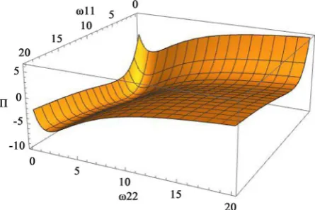
The multifrequency second order test for the discussed complex system with the inven-tory interactions is shown on Figure 1 and Figure 2 for different number of harmonics.

The second order test obtained shows the diversified advantageous operation fre-quencies for particular subsystems ω =1 5.5 and ω =2 2.5 for the single harmonic and

1 4.5

(10)

[image:10.595.247.502.71.215.2]

Figure 1. The single harmonic second order test for the complex sys-tem with the inventory interactions.

Figure 2. The five harmonics second order test for the complex

sys-tem with the inventory interactions.

5. Conclusion

In this note, we formulated the optimal multiperiodic control problem for inventory constrained subsystems. It is aimed at the intensification of the productivity of complex processes. We proposed a multifrequency second-order test for complex multiperiodic systems including the boundary optimal steady-state process and an arbitrary large number of harmonics used to verify its improvement by the multiperiodic operation. We generalized the method of critical directions for single periodic systems [10][11] to complex multiperiodic systems. We illustrated the approach proposed on the example of the multiperiodic optimization of a system of chemical reactors.

Acknowledgements

This work has been supported by the National Science Center under grant: 2012/07/B/ ST7/01216.

References

[image:10.595.262.485.256.404.2]

(11)

Engineering, 2009, Article ID: 137483. http://dx.doi.org/10.1155/2009/137483 [2] Colonius, F. (1988) Optimal Periodic Control. Springer-Verlag, New York.

http://dx.doi.org/10.1007/BFb0077931

[3] Gräber, M., Kirches, Ch., Bock, H.G., Schlöder, J.P., Tegethoff, W. and Köler, J. (2011) De-termining the Optimum Cyclic Operation of Adsorption Chillers by a Direct Method for Periodic Optimal Control. International Journal of Refrigeration, 34, 902-913.

http://dx.doi.org/10.1016/j.ijrefrig.2010.12.021

[4] Skowron, M. and Styczeń, K. (2006) Evolutionary Search for Globally Optimal Constrained Stable Cycles. Chemical Engineering Science, 61, 7924-7932.

http://dx.doi.org/10.1016/j.ces.2006.09.005

[5] Silveston, P.L., Budman, H. and Jervis, E. (2008) Forced Modulation of Biological Processes: A Review. Chemical Engineering Science, 63, 5089-5105.

http://dx.doi.org/10.1016/j.ces.2008.06.017

[6] Hernandez-Martinez, E., Granados-Focil, A., Meraz, M. and Alvarez-Ramirez, J. (2011) Analysis of Periodic Operation of Bioreactors from a First-Harmonic Balance Approach. Chemical Engineering and Processing: Process Intensification, 50, 1169-1176.

http://dx.doi.org/10.1016/j.cep.2011.09.001

[7] Dzyadyk, V.K. (1977) Introduction to the Theory of Uniform Approximation of Functions by Polynomials. Naukova Dumka, Kiev. (In Russian)

[8] Styczeń, K. (1986) Trigonometric Approximation of Optimal Periodic Control Problems. International Journal of Control, 43, 1531-1542.

http://dx.doi.org/10.1080/00207178608933557

[9] Ben-Tal, A. (1980) Second-Order and Related Extremality Conditions in Nonlinear Pro-gramming. Journal of Optimization Theory and Applications, 31, 143-165.

http://dx.doi.org/10.1007/BF00934107

[10] Bernstein, D.S. (1984) A Systematic Approach to Higher-Order Necessary Conditions in Optimization Theory. SIAM Journal on Control and Optimization, 22, 211-238.

http://dx.doi.org/10.1137/0322016

[11] Bernstein, D.S. (1985) Control Constraints, Abnormality, and Improved Performance by Periodic Control. IEEE Transactions on Automatic Control, AC-30, 367-376.

(12)

Submit or recommend next manuscript to SCIRP and we will provide best service for you:

Accepting pre-submission inquiries through Email, Facebook, LinkedIn, Twitter, etc. A wide selection of journals (inclusive of 9 subjects, more than 200 journals)

Providing 24-hour high-quality service User-friendly online submission system Fair and swift peer-review system

Efficient typesetting and proofreading procedure

Display of the result of downloads and visits, as well as the number of cited articles Maximum dissemination of your research work

Submit your manuscript at: http://papersubmission.scirp.org/