The Thirty-First AAAI Conference on Innovative Applications of Artificial Intelligence (IAAI-19)
Early-Stopping of Scattering Pattern Observation with Bayesian Modeling
Akinori Asahara, Hidekazu Morita
Hitachi Ltd.Tokyo, 100-8280, Japan
Chiharu Mitsumata
National Institute for Materials ScienceTsukuba, 305-0047, Japan
Kanta Ono
High Energy Accelerator Research Organization Tsukuba, 305-0801, Japan
Masao Yano, Tetsuya Shoji
Toyota Motor CorporationToyota, 471-8572, Japan
Abstract
This paper describes a new machine-learning application to speed up Small-angle neutron scattering (SANS) exper-iments, and its method based on probabilistic modeling. SANS is one of the scattering experiments to observe mi-crostructures of materials; in it, two-dimensional patterns on a plane (SANS pattern) are obtained as measurements. It takes a long time to obtain accurate experimental results be-cause the SANS pattern is a histogram of detected neutrons. For shortening the measurement time, we propose an early-stopping method based on Gaussian mixture modeling with a prior generated from B-spline regression results. An experi-ment using actual SANS data was carried out to examine the accuracy of the method. It was confirmed that the accuracy with the proposed method converged 4 minutes after starting the experiment (normal SANS takes about 20 minutes).
Introduction
Materials informatics (MI) is a field in which information technology is used to accelerate materials science research. Especially data mining techniques will be used to easily find very small features of measurement data. As a such appli-cation, we propose an approach to shorten the time for ex-periments by making predictions based on machine learn-ing. Imagine an experiment that usually takes 10 minutes, where half of the results are obtained in 5 minutes. If the full results of the experiment can be predicted with the data obtained in 5 minutes, the experiment can be finished imme-diately; namely, the experiment can be made twice as fast. Moreover, if the prediction requires only 1 minute, it will be ten times faster. Generally speaking, measurements on materials requires a special facility and cost a lot – if it is based on high-energy physics, the cost is comparable with hundreds of millions of dollars. Accordingly, such precious experiment time have to be efficiently used.
This study focuses on small-angle neutron scattering (SANS) experiments(Higgins and Benoˆıt 1994). SANS is a scattering experiment that is a popular method for observing the microstructures of materials. There are similar various scattering experiments such as x-ray scattering, ion-beam scattering, etc. Their difference lies just in the particles to be scattered. The solution for the problem in SANS can be
Copyright c2019, Association for the Advancement of Artificial Intelligence (www.aaai.org). All rights reserved.
Neutron beam
Material sample
Detector plane Source
0 0 0 0 0 1 1 2
1 0 0 4 1 0
0 4
2 5
5 8
2 0 5 8 10
1 0 2 0
0 0 3 0
1 1
1 0
2 1 1
0 1 0 1
1 0
2 3
5 0 0 0 0 1 0
2 0
1 1
0 0 0 0 0
SANS pattern
𝜃 𝐿
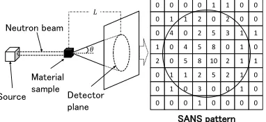
Figure 1: SANS Experiment
expected to apply for these experiments also. Thus the prob-lem is crucial enough to be solved.
We accordingly propose a method to predict a SANS pat-tern in a short time. The method is based on the Gaussian mixture model (GMM). The GMM can be fitted to the SANS pattern through the variational Bayesian (VB) approach. In particular, our method can estimate the accuracy of the pre-diction, and thereby, the SANS experiment can be stopped once the prediction is deemed accurate enough. If it stops be-fore convergence of the SANS pattern, the experiment will be faster.
Problem Setting
Overview of SANS
Figure 1 shows an illustration of the experimental instru-ments. A neutron beam incident upon sample interacts with the microstructures therein. The directions of the neutrons thus are changed due to the interactions. The angle θ be-tween a straight beam and the changed direction of the scat-tered beam depends on the interaction.
The neutrons detectors are arranged on a plane. When the distanceLbetween the sample and the plane is large enough, the coordinate values on the planex = (x, y)are approxi-mately in proportion toLsinθ 'Lθ. The probability den-sity function (PDF)P(x)of neutron detection corresponds to the probabilityP(θ)that neutron goes in the direction of θ, which is related to the microscopic structures.
Hence,P(x)is crucial for understanding the microstruc-ture of the material. When n detection events denoted as
{x1,x2,· · ·,xn} are obtained, the “true” PDFP(x)is to
coor-dinates are discrete, depending on the density of the detec-tors. Therefore, the event data are usually handled as event counts in a certain time duration t for each detector (de-noted as{vi,j(t)}, where(i, j)is discretizedx), as shown
by the “SANS pattern” in the figure. Furthermore,{vi,j(t)}
is considered to be a histogram. Hence, vi,j(t)/Pvi,j(t)
will converge to the true probabilityPi,j that is derived by
taking the integral ofP(x)over the cell(i, j). Accordingly, the true PDFP(x)is estimated from the histogram{vi,j}
after a sufficiently long time.
Fast SANS with Prediction
The prediction-based early-stopping for SANS (hereafter, called fast SANS) is proposed in this paper. For the early-stopping, the SANS pattern{vi,j(t)}is periodically posted
to a computer to predictPi,j = limt→∞vi,j(t)/Pvi,j(t)
with {vi,j(t)} and tests whether the prediction result has
converged. If it has converged, the computer sends a ter-mination signal to the experimental instrument. Otherwise, the computer waits for the next SANS pattern. Note that the prediction and convergence test have to be fast to terminate the experiment earlier. If it takes more time than the con-ventional SANS, the fast SANS cannot be said to be not fast. For example, if the conventional SANS takes 20 min-utes, the time for the process should be less than 20 minutes. Even if the time for the process is 10 minutes, there is just one chance to send the termination signal.
According to the discussion, the problem to be solved is that of predicting the true PDF obtained as Pi,j = limt→∞vi,j(t)/Pvi,j(t)under the following constraints.
1. Only{vi,j(τ)}wheret > τ are available for the
predic-tion
2. The convergence of the PDF can be evaluated
3. The processing time to obtain the PDF should be short 4. The PDF formula may be smooth, but must be general In this paper, probabilistic modeling is discussed as an ap-proach to solve the problem.
Related Works
Scientific data is one of the targets of study in the data en-gineering field. Compressed sensing(Donoho 2006)(Bour-guignon, Carfantan, and B¨ohm 2007)is a popular technology for reconstruction by sparse modeling of a few data. Com-pressed sensing assumes that the signal sources are sparsly distributed. Under the constraint of sparsity, a compressed sensing model can be accurately estimated without many sensing data. In such case, we can reduce the sensing data without loss of accuracy. Here, compressed sensing has been used to accelerate the measurements(Lustig et al. 2008). On the other hand, while smoothness is suitable for fast SANS, sparsity might be unsuitable for it.
The goal of the prediction is also similar to those of image reconstruction and restoration methods. A popular method for image restoration is the random Markov filed(Zhang 1993). It might be applied to the SANS pattern, though the result is not likely to be so accurate because the restoration is developed for visually improving the images.
Kernel density estimation (KDE)(Silverman 1986)(Si-monoff 1996) is also a well-known method to estimate a smooth distribution for point-like events. In KDE, every ob-served point is inferred to have a probability around it. The effect is determined by the “kernel function”, of which the parameter is the distance from the observed pointxn. The PDFP(x)is formed as the sum of the contributions as fol-lows.
P(x) = 1
hN
N X
n
K(|x−xn|
h ), (1) wherexn is thenth observed point,his a bandwidth pa-rameter to indicate the effective area of a point, andNis the number of points. A Gaussian functionN(x|xn, hI)is of-ten used as the kernel function for generality, whereIis the unit matrix andxnis thenth observation.
A criterion to determine termination of the experiment is required for fast SANS. To evaluate the convergence of the PDF, a simple criterion is how much the PDF was changed. For KDE, the difference between the latest PDF and the pre-vious one should be calculated as the criterion. The criterion CKDE(t)at timetis derived as follows.
CKDE(t) =
Z
|P({x1,· · ·xt})−P({x1,· · ·xt−1})|dx.
(2) A disadvantage of this criterion is the timing for detecting convergence. Namely, the criterion can detect convergence only after the PDF has converged. For a fast SANS experi-ment, the detection of the convergence should be simultane-ous with convergence. Convergence of the parameter might be used as a criterion for GMM modeling, instead of a PDF. However, in this case as well, convergence is detected after convergence.
GMM-based prediction
Bayesian Early-stopping
In this study, Bayesian estimation approach is taken to obtain a criterion for the convergence of the PDF. In the Bayesian approach, the parameters of the PDF, denoted as {η}, are also probabilistic, in addition to observations{x}. The PDF of the parameters {η} when {xn} are given is denoted as P({η}|{xn})hereafter. The basic idea of the proposed method is that the variance ofP({η}|{xn})is used as the criterion of experiment termination because the PDF indi-cates the uncertainty of{η}.
Two requirements, i.e., high accuracy and short pro-cessing time, should be satisfied for a fast SANS ex-periment. Both accuracy and processing time depend on the prior setting. If a prior similar to the P({η}|{xt}) is
used,P({η}|{xt})is considered to converge earlier. In the proposed method, P(x) is roughly estimated before the Bayesian estimation, and the prior is constructed along the roughly estimatedP(x).
Variational Bayesian Estimation for GMM
P({η}|{xn}). VB estimation approximately assumes that the prior of the GMM parameters is independent from the distribution of the latent parameters. Under this assumption, the PDF estimation is separated into two steps: estimation of the latent parameter and improvement of the PDF of the parameters. The whole process is called the Bayesian EM algorithm(Bishop 2006).
The PDF of the GMM for fast SANS is as follows. P(x|{πk},{µk},{Λk}) =
X
k
πkN(x|Λk, µk), (3)
wherexis a point on the detection plane,N(x|Λk, µk)is the
k-th two-dimensional Gaussian function with a correlation matrix denoted byΛk and an average denoted byµk.πk is
the mixing ratio of thekth component. The priors for the parameters{πk},{µk},and{Λk}are set
P({πk},{µk},{Λk} |W0, ν0, β0)
= Dir({πk}|α0)
Y
k
N(µk|(β0Λk)−1,m0)W(Λk|W0, ν0).
α0, W0, ν0, and β0 are the given parameters of the prior
(called hyper-parameters). W(W, ν) is the function called the Wishart distribution with the deviationW and degrees of freedomν.Dir({π}|α)is the Dirichlet distribution with parameterα.
For the Bayesian estimation, a posterior with new obser-vations{xn}is calculated. If the prior mentioned above is used, the formula of the posterior is the same as that of the prior. That is to say, the hyper-parameters α0, β0,m0, W0
are revised through Bayesian estimation.
αk=α0+Nk, βk=β0+Nk, (4)
mk=
1
βk(β0m0+Nkx¯k), νk=ν0+Nk, (5)
Wk−1=W0−1+SkNk+ Nkβ0 Nk+β0
(m0−¯xk)(m0−x¯k)T, (6)
whereNk,xk, andSk are respectively calculated as
Nk= X
n
rn,k, ¯xk= 1
Nk X
n
rn,kxn, (7)
Sk = X
n
rn,k(xn−xk¯ )(xn−xk¯ )T. (8)
rn,k, which is called ”responsibility”, is calculated as
rn,k=
ρn,k P
nρn,k
, (9)
ρn,k≡π˜k|Λ˜k| 1 2e
h −βk2 −1
2(xn−mk)TWk(xn−mk) i
, (10)
ln ˜πk ≡lnψ(αk)−lnψ( X
k
αk), (11)
ln|Λ˜k| ≡lnψ(
νk
2 ) + lnψ(
νk−1
2 ) + ln 4|Wk|, (12)
whereψ(·)is a digamma function. The responsibilityrn,k
indicates the contribution to each component labeled by k. The calculation of the responsibility requires the hyper-parameters; however, the hyper-parameter estimation also
Relative
frequency
X
Figure 2: PDF distribution
requires the responsibility. So, the above-described pro-cesses are iterated to optimize the hyper-parameters. After iterating the calculation, the optimized hyper-parameters are obtained.
The probability distribution is estimated with marginal-ization of every hidden parameter,
P(x) =
Z X
z
P(x|µk,Λk)P(z=zk|{πk})
×Pk(µk,Λk|mk, βk, Wk, νk)P({πk}|{αk})dπdΛdµ.
(13) The integration can be carried out as follows.
P(x) =
P
kαˆkSt(x|mˆk, L(βk, νk, Wk),νˆk−1) P
k0αˆk0
, (14)
where
L( ˆβk,νˆk,Wˆk)≡
(ˆνk−1) ˆβk
1 + ˆβk ˆ
Wk. (15)
Criteria for Terminating the Experiment
In the Bayesian approach, the PDF of the parameters is esti-mated and predicted SANS pattern is derived with marginal-ization of it, as shown above. The relation between probabil-ity and the observations of the SANS pattern is illustrated in Fig. 2. If the observations shown as a histogram are input, the PDF of the parameters is determined. Various PDFs of new observations can be estimated depending on the PDF of the parameters. Through merginalization, the average of such PDFs is calculated for predictingx(drawn as the solid line). That is, the expectation value ofP(x)shown in for-mula (13) is written as
P(x) =EπΛµ X
z
P(x|µk,Λk)P(z=zk|{πk}) !
(16)
whereEπΛµ is the expectation value overπΛµ. However,
the other PDFs such as those indicated by the dashed line and the dotted line in the figure are possible estimates. The variance of the probability, therefore, is considered to be a criterion for predicting convergence.
The variance of the probability is similarly calculated as
E(P(x)2)−E(P(x))2. The first term is written as a sum of
componentsFi,j.
E(P(x)2) =X i,j
Z
P(x|µi,Λi)P(x|µj,Λj)P(z=zi|{πi})
×P(z=zj|{πj})dπdΛdµ≡X
i,j
The integrations in Fi,j are categorized into two types.
When the two indices are the same, as inFk,k, we have
Fk,k=
αk(αk+ 1) P
iαiPj(αj+ 1) ×
1 4π|W|
1
2(ν−1)St(x|mˆk, L(1 2 ˆ
βk,νˆk+ 1,2 ˆWk), νk).
(18) If the two indices are different, we have
Fij =
αiαj P
l,mαl(αm+ 1)
St(x|mˆi, Li,νˆk−1)St(x|mˆj, Lj,νˆj−1). (19)
Moreover,E(P(x))2 is similarly described as a sum of
components.
E(P(x))2=X i,j
ˆ αiαjˆ (P
ˆ
αk)2St(x|mˆi, L(βi, νi, Wi),νiˆ −1)
×St(x|mj, Lˆ (βj, νj, Wj),νjˆ −1) =X i,j
˜
Fi,j (20)
The formulas ofFi,j andF˜i,j are very similar. Actually,
ifNk→ ∞, we have
Fi,j'
αiαj
(P iαi)
2N(x|mˆi, L(βi,νˆi,Wˆi))
× N(x|mˆj, L(βj,νˆj,Wˆj))'F˜i,j. (21)
Thus,F˜i,j−Fi,j → 0whenNk is large enough. Because
Nk becomes larger when the data increase, this proves that
the variance will be 0 whent→ ∞.
B-spline-based Rough Estimation of Priors
As mentioned above, {m0, β0, W0, ν0, α0} are the
hyper-parameters for the GMM. If there are enough observations, these hyper-parameters are determined optimally. However for fast SANS, the number of iterations of the VB estima-tion is limited because the process should finish before the next SANS patterns arrive. Thus, a rough estimate of the PDF is used to generate more suitable priors in the proposed method.
The rough estimation is a regression estimation with multinomial functions, i.e., B-spline curves(Silverman 1985). A B-spline curve is a combination of multinomial functions, determined by given parameters that correspond to points, called control points. Thus, the control points should be optimized to fit the PDF to the SANS patterns.
The estimated PDFP(x)with B-spline curves is used for generating the prior for the VB estimation. If the gradient of the estimated function is higher, more Gaussian functions of GMM will be required. So in the proposed methods, more components of the Gaussian priorm0should be generated
in the area where the gradient is high. Namely m0 is
se-lected randomly with the probability that is in proportion to the strength of the gradient|∇P(x)|. Even if the number of components is limited due to processing time, we can select a prior suitable for the posterior.
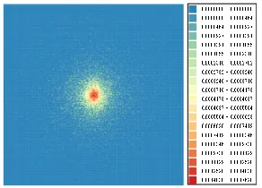
Figure 3: SANS pattern after 1 minute
・・・ ・・・
・・・
90 min 1 min 2 min 3 min
Test data (90 min) Training data (90 min)
Figure 4: Expeimental data setting
Experiments
Experimental Settings
Experiments using actual SANS data were carried out to ex-amine the accuracy of the proposed method, that is, GMM with B-spline-based prior. The data for the experiment were from an actual SANS experiment lasting 180 minutes (called the “180min SANS pattern” here). The sample for the exper-iment was a polycrystalline metallic sample, for which gives SANS patterns are intense at the center. The SANS pat-tern consists of 256×256 cells with intensity. The 180min SANS pattern was divided into 180 patterns that included the observations accumulated in 1 minute. Figure 3 shows one of these patterns (called a “1min SANS pattern”). By aggregating x 1-min SANS patterns, we can generate an “x min SANS pattern” freely. The measurement normally takes 20 minutes to obtain accurate SANS patterns. For the exper-iments, the 1-min SANS patterns were grouped into two sets of 90 patterns, as illustrated in Fig 4. The 90 patterns of one set were aggregated to make a “true” data. The patterns of the other set were used as inputs to the prediction methods.
The accuracies of KDE and GMM with the VB estimation (called simply GMM) were evaluated against those of the proposed method, that is, GMM with B-spline-based prior (called BSGMM). The logarithmic likelihood, expressed as
P
tlnP(xt), was used as the criterion for accuracy.
Hyper-parameters of the methods have to be determined before the evaluation. For the VB estimation of GMM, they were set naive values, that is,m0 =0,β0 = 1.0,W0 =I,ν0 =0,
α0= 0, and the number of mixed components was 50. The
BSGMM estimation was carried out with the same settings exceptm0.
-9.036 -9.034 -9.032 -9.03 -9.028 -9.026 -9.024
0 2 4 6 8 10 12
Lo
ga
ri
th
m
ic
li
ke
li
h
o
o
d
SANS-experiment duration [min] BSGMM GMM KDE
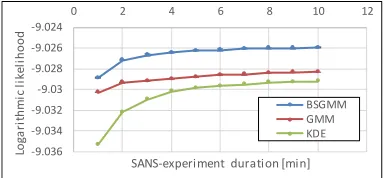
Figure 5: Accuracy in experiment 2
and8, the accuracy ofh= 4was better than those ofh= 6
and8. The accuracy ofh= 2results were lower thanh= 4
before 4 min SANS pattern was input. However, the initial behavior is crucial for fast SANS because the idea is for the experiment to finish earlier. Thus, h = 4was considered most reasonable for fast SANS.
Generally speaking, the iteration processes for the VB es-timation should continue until convergence. However pro-cessing time is limited for the fast SANS. Thus to keep the processing time sufficient for fast SANS, the number of the iteration was set to constant. So the number of the iterations in VB estimation was adjusted to 400 manually to finish the process in 1 minute. Additionally, KDE was also tuned. If
|x−xn| > 3σ, the kernel function was set to 0. The
ef-fects in such case were quite small, so the calculation can be omitted to finish the calculation in 1 minute.
The CPU of the computer used in the experiment was Intel Core i7-3770 3.40 GHz and the RAM was 8GB. The meth-ods were implemented in Java using JDK 1.8.0 update 144 and multithreading.
Experimental Results
Figure 5 plots the accuracy of the prediction by BSGMM, GMM and KDE (h= 4). The vertical axis indicates the log-arithmic likelihood and the horizontal axis is the duration to obtain SANS pattern. BSGMM and GMM are calculated 10 times with changing the random seeds and the averages are plotted in the figure. The error bars indicating the standard errors among them are drawn but they are invisibly small. The accuracy of BSGMM is highest; that of GMM is sec-ond; that of KDE is lowest.
For comparison, the accuracy of the conventional method was evaluated. The relative frequency of the SANS pattern is used as the probability, where the probability is set to
10−200 at points of which the probability is 0 to avoid in-finity to avoid∞due tolog 0. The accuracy at 1minute was -138.5 and that at 10 minutes was -36.1. With the conven-tional method, it is generally considered that it takes around 20 minutes for convergence. In contrast, the BSGMM and GMM almost converged at only 4 minutes. This indicates that GMM and BSGMM can shorten the SANS experiment duration from 20 minutes to 4 minutes.
Figure 6 plots the average of the processing time for each method. The process was carried out 10 times and the av-erages are plotted with the error bar indicating the standard error. All of the calculation were finished in 60 seconds
be-0 10 20 30 40 50 60
0 2 4 6 8 10 12
C
a
lc
u
la
tio
n
ti
m
e
[s
ec
]
SANS-experiment duration [min]
BSGMM GMM KDE
Figure 6: Processing Time in experiment 2
-80% -70% -60% -50% -40% -30% -20% -10% 0% 10%
0 2 4 6 8 10 12
C
o
n
ve
rg
en
ce
-c
ri
te
ri
a
d
ec
re
a
se
ra
te
SANS-experiment duration [min]
BSGMM GMM KDE
Figure 7: The differential convergence criteria
cause of the tuning. The calculation time of GMM and BS-GMM are rising up after 4 minutes, but it keeps around 50 seconds. Thus the processes can be carried out in 1 minute, which is period of SANS pattern. The result shows that the GMM and BSGMM are feasible for the fast SANS.
Additionally the criteria of convergence for each method were evaluated. For KDE,CKDE defined as formula (2) is
sutiable. As the discretized and normalized version of it, the average difference between thetandt−1results were the criteria. For GMM and BSGMM, formula (20) was the cri-teria. Figure 7 plots decrease rates of them (difference be-tween the criteria attandt−1was divided by the criteria att= 0). The criteria are basically correlated to the accura-cies; however according to its criteria, KDE did not converge until around 8 minutes. In contrast, the GMM criteria were almost constant after 3 or 4 minutes. Therefore, the crite-ria are feasible for judging convergence, and the GMM and BSGMM criteria are the best.
Discussion
Figures 8 show the predicted patterns using 1-min SANS pattern and the original SANS pattern. The GMM and BS-GMM results are smoother than the KDE result. This im-plies that the number of data is too small for KDE to give an estimate. To obtain smoother results with KDE, the band-width has to be larger, but a larger bandband-width flattens the SANS pattern. As shown, GMM and BSGMM are compa-rably smooth, though BSGMM result is not symmetric. This asymmetry comes from the asymmetry of the prior.
ver-(a) KDE result (b) GMM result (c) BSGMM result
Figure 8: Predicted SANS patterns
-5 -4 -3 -2 -1 0 1
0 0.5 1 1.5 2
d
lo
g10
(P
rb
a
b
ili
ty
)/d
lo
g10
(r
)
log10(r)
Truth BSGMM GMM KDE4
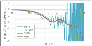
Figure 9: Differential Cross Section aty= 128,128< x
tical axis is the differential oflog10P as follows.
log10P(xn)−log10P(x0)
log10|xn−xc| −log10|x0−xc|
, (22)
wherexn = (n+ 128,128)andxc = (128,128). Because KDE is based on smoothing, the results of KDE tend to be flat. Thus, the differential values of KDE are nearer to zero than those of GMM and BSGMM. The truth is actually sim-ilar to the GMM and BSGMM results.
The truth frequently oscillates at highlog10r. The oscilla-tion is caused by the inaccuracy of the SANS pattern. KDE similarly oscillates because the PDF is generated from the detected events. In contrast, GMM and BSGMM do not os-cillate unlike KDE. As the result, we can see a peak around
log10r = 1.3, which implies that there are effects from the microstructure around the scale. GMM and BSGMM are hence superior in this aspect.
As discussed above, both GMM and BSGMM are appli-cable for fast SANS. However remember that BSGMM is more accurate than GMM as shown Fig. 5. Therefore it is considered that BSGMM is more appropriate than GMM.
Conclusion and Future work
A GMM with B-spline-based prior for fast SANS exper-iments was proposed in this paper. An experiment using actual data confirmed that the GMM-based prediction of SANS patterns requires only a few minutes worth of SANS data to predict the results that will be obtained later. The accuracy converged 4 minutes after starting the experiment; this compares favorably with the around 20 minutes for con-ventional SANS experiments. Therefore, we conclude that the proposed method shortens the SANS experiment to 1/5th of its usual duration.
SANS is just one of many scattering experiments. That is, there are many scattering-like experiments in materi-als science: light scattering (such as X-ray scattering and laser scattering), beam scattering (such as ion-beam scatter-ing and electron-beam scatterscatter-ing), and so on. The proposed method may be applied to such experiments. Not only that, the problem that spatial distribution of events should be es-timated fast is common in statistics survey. Modifying it for those applications will be a future work.
References
Attias, H. 1999. Inferring parameters and structure of la-tent variable models by variational bayes. InProceedings of the Fifteenth conference on Uncertainty in artificial intelli-gence, 21–30. Morgan Kaufmann Publishers Inc.
Bishop, C. M. 2006. Pattern Recognition and Machine Learning. New York: Springer.
Bourguignon, S.; Carfantan, H.; and B¨ohm, T. 2007. Spar-spec: a new method for fitting multiple sinusoids with irreg-ularly sampled data.Astronomy & Astrophysics462(1):379– 387.
Donoho, D. L. 2006. Compressed sensing. IEEE Transac-tions on information theory52(4):1289–1306.
Higgins, J. S., and Benoˆıt, H. 1994. Polymers and neutron scattering. Clarendon press Oxford.
Lustig, M.; Donoho, D. L.; Santos, J. M.; and Pauly, J. M. 2008. Compressed sensing mri. IEEE Signal Processing Magazine25(2):72–82.
Silverman, B. W. 1985. Some aspects of the spline smooth-ing approach to non-parametric regression curve fittsmooth-ing. Journal of the Royal Statistical Society. Series B (Method-ological)1–52.
Silverman, B. W. 1986. Density Estimation for Statistics and Data Analysis. Chapman and Hall/CRC.
Simonoff, J. S. 1996. Smoothing methods in statistics. Springer.
Waterhouse, S. R.; MacKay, D.; and Robinson, A. J. 1996. Bayesian methods for mixtures of experts. InAdvances in neural information processing systems, 351–357.