Methods in Oil Recovery Processes and Reservoir Simulation

ISSN Online: 2160-0406 ISSN Print: 2160-0392

Methods in Oil Recovery Processes and

Reservoir Simulation

Pablo Druetta

1

, Pietro Tesi

2

, Claudio De Persis

2

, Francesco Picchioni

1

1_{Department of Product Technology, ENTEG, University of Groningen, Groningen, The Netherlands}

2_{Department of Smart Manufacturing Systems, ENTEG, University of Groningen, Groningen, The Netherlands}

Abstract

The exploitation of an oil field is a complex and multidisciplinary task, which de-mands a lot of prior knowledge, time, and money. A good reservoir characterization is deemed essential in the accomplishment of Enhanced Oil Recovery (EOR) pro- cesses in order to estimate accurately the properties of the porous medium affecting the flow properties. Several techniques at a field scale are currently being used to de-termine these properties, which are time and money consuming. But these alone do not guarantee the success of the project. Reservoir simulation and numerical tech-niques were then included in the pre-development and follow-up studies as an effec-tive tool to determine the productivity and future behavior of the oil field. As the computational power increased, more advanced and detailed models were developed, including different chemical and physical phenomena. But alongside this process, there was an active research in the area of reservoir simulation, improving the accu-racy and efficiency of the numerical schemes used for the flow, transport, and energy equations. The aim of this review is to address the topics described. Firstly, the origin of an oil recovery process, the economic factors and field tests involved are intro-duced. Secondly, the oil and porous medium origin and characterization as well as an introduction to the fundamental concepts and equations are associated to reservoir simulation. Finally, a brief description and analysis of the techniques are used in re-servoir simulation employing finite difference methods, their downsides and possible ways to overcome these problems.

Keywords

Petroleum Engineering, Enhanced Oil Recovery, Reservoir Simulation, Numerical Analysis

How to cite this paper: Druetta, P., Tesi, P., De Persis, C. and Picchioni, F. (2016) Me- thods in Oil Recovery Processes and Re- servoir Simulation. Advances in Chemical Engineering and Science, 6, 399-435.

http://dx.doi.org/10.4236/aces.2016.64039

Received: August 30, 2016 Accepted: October 9, 2016 Published: October 12, 2016 Copyright © 2016 by authors and Scientific Research Publishing Inc. This work is licensed under the Creative Commons Attribution International License (CC BY 4.0).

http://creativecommons.org/licenses/by/4.0/

1. Oil Origin and Formation

1.1. Introduction

The era of discovery and subsequent exploitation of the denominated “easy oil” (part of the so called conventional reserves) is over [1]-[5]. After primary and secondary recov-ery, oil companies have begun with more complex Enhanced Oil Recovery (EOR) processes involving fluids or chemical reactions that require a greater detail of the phenomena taking place in the porous medium. In addition to these complications there exist non-technical related factors that might increase the risk of an investment

[6]. An example of this may be the development of off-shore platforms, plants located in remote areas of the world or the exploitation of unconventional deposits (heavy oil, shale oil, tar sands). All these projects require a prior investment (in the order of several tens of millions of dollars high risk projects), so companies make use of several tech-niques in the stage of feasibility analysis to limit this risk and increase the chances of success of the operation (Figure 1) [7][8].

[image:2.595.198.550.441.676.2]

These techniques, used to predict and optimize the exploitation, include laboratory and field tests (e.g. seismic 2D/3D/4C before starting operations and 4D to follow up the changes during exploitation, geostatistics) to give an idea of the conditions of the porous medium and its production performance [9]-[13]. However, these tools have proven to be insufficient [12][14][15] and therefore oil companies have begun using computational tools to predict and optimize their projects and production facilities, which is known as Reservoir Simulation. The latter consists in solving numerically the differential equations describing the fluid flow in porous media, which have no analyti-cal solution, taking into account all geologianalyti-cal, physianalyti-cal, chemianalyti-cal and/or mechanianalyti-cal

phenomena occurring during operation so as to analyze and predict behavior as a func-tion of time. The reservoir simulafunc-tion can be used as well in inverse engineering prob-lems for optimizing existing numerical models and couple the dynamic/historic data (production) in the simulation [15]-[18].

Generally speaking, reservoir simulation consists of three main parts: the physical characterization of a geological model describing the rock formation; a model characte-rizing the fluid flow and finally “well models” which describe the conditions under which fluids are injected or extracted from the reservoir [19]. The latter, along with the wellbore and the primary surface facilities, constitutes what is known as upstream. During the last 30 years numerous theoretical and practical advances have been devel-oped due to the appearance of new numerical techniques and increased computational power, respectively [15][20]. This led to a new generation of more complex and de-tailed models. The accurate representation of the reservoir and the fluid contained in it is an issue that still needs to be more carefully addressed in order to reduce risks in ex-ploration and production (E&P) projects. One of the most important points is related to the scales of the models: current grids are still large when compared to the geological characterization, description of chemical processes or fluid flow. Most of current nu-merical models used in reservoir simulation may contain from 105 _{to 10}8 _{grid blocks,}

depending on the model type, complexity, computational power available and fluid be-havior.

The development of increasingly complex and detailed models requires the use of numerical techniques to solve these at reasonable times. Moreover, the representation of the properties of the porous medium and the characteristics of crude oil and natural gas at high pressures and temperatures may differ from laboratory tests, causing dif-ferences between the results and simulation. Another important topic is how to assess and properly estimate the properties of the rock formation. Geologists use statistical techniques in order to recreate the model properties of a porous medium, which are determined by several tests (e.g. seismic studies, drill core samples and even production data). However, other numerical tools are required (e.g. Monte-Carlo or Stochastic Processes) to take into account the effects of uncertainties in the model [21][22].

The aim of this review is to briefly describe the characterization of porous media and its main parameters. Then, models governing fluid flow in porous media are intro-duced. This consists in Darcy’s equation and the more complex compositional model for multiphase flow (where the component transfer between phases introduces nonli-nearities in the mass transport equation), which is useful to describe chemical EOR op-erations. The second part comprises a brief explanation of the numerical methods used as well as the problems associated with these schemes (numerical dispersion and dissi-pation), and possible solutions using advanced numerical schemes.

1.2. Origin of the Oil

porous medium is generally considered of sedimentary origin and consists of a series of microchannels (about 1 - 100 microns diameter) interconnected where these fluids can flow (Figure 2). These formations may have some tens of meters thickness, but may extend several kilometers in the lateral directions [23].

The origin of crude oil prior to the migration and deposit of hydrocarbons in the porous media is also a long and complex process [25]-[27]. The source of hydrocarbons consists of a series of phenomena, both organic and inorganic, taking place during long periods of time (in the order of million years) [28]. Most of these hydrocarbons origi-nate in organic decomposition processes. The first stage (called diagenesis) involves the sedimentation of remains of dead plants and animals. Under these conditions, at low depths, the action of bacteria produce methane, water and CO2, leaving as reaction

products of kerogen substances (cyclic and large hydrocarbon molecules containing oxygen, nitrogen and sulfur). The second process, called catagenesis, occurs at greater depths and temperatures. In this region, known as the oil window zone, the kerogen molecules break in smaller, heavy hydrocarbons forming the oil phase. At higher tem-peratures the cracking of hydrocarbons continues creating lighter compounds, first wet gas and subsequently dry gas. Finally, at even greater depths, the last process takes place (called metagenesis), where the remaining kerogen is out of hydrocarbons and subse-quent cracking processes terminate when there is no hydrogen in the compound. The result of these reactions is the formation of graphite (Figure 3).

1.3. Porosity and Permeability

[image:4.595.195.554.532.687.2]

A porous rock formation is composed of a solid part, called solid matrix, and the re-maining void space or microchannels whereto oil migrates [31]. The volumetric frac-tion of these channels is denominated porosity of the porous media. The latter depends on the fluid pressure, if the rock is compressible, or in some other phenomena which may take place (e.g. adsorption of chemical components during EOR processes). The following list provides typical values of porosity according to the origin of the rock formation [32][33]: Consolidated sandstones 0.05 to 0.3; limestones 0.1 to 0.4; uniform spheres with minimal porosity packing 0.25; uniform spheres with normal packing

[image:5.595.47.547.67.466.2]

Figure 3. Origin of oil (adapted from [29][30]).

0.35; unconsolidated sands with normal packing 0.40 and unconsolidated clays 0.60. The permeability of the formation is a property that characterizes the ease with which fluids can flow when a pressure gradient is applied between two points. None-theless, reservoir rocks usually have no uniformity in their properties because of the mechanisms involved on its formation, thus the permeability will have a large dispersity in its values [34][35]. The fluids used commonly in EOR operations, more mobile than oil, occupy the high-permeability zones (e.g. faults or fractures), with the result that large areas of oil will be bypassed, reducing the efficiency of the process. Mathematical-ly, the permeability can be expressed as a diagonal tensor (K). When the medium is isotropic then the permeability can be represented as a scalar function. Due to transi-tions between different rock types, the permeability may vary swiftly throughout the reservoir, going from extreme low permeability areas of 1 mD to areas with permeabili-ties exceeding 10 D.

estab-lished several restrictions: the whole void space of the porous medium is intercon-nected; the mean free path length of the fluid molecules or molecules contained in the fluid must be negligible when compared to the dimensions of the pore channels, and the dimensions of the void space must be small enough so that the fluid flow is con-trolled by adhesive forces at fluid-solid interfaces and cohesive forces at fluid-fluid in-terfaces (in multiphase systems) [31]. These assumptions allow excluding any discon-nected channels in which there can be no fluid flow, eliminating the difference between the concepts of total porosity and effective porosity. Furthermore, since the dimensions of the molecules or particles in the fluid are negligible with respect to the microchan-nels, a suitable replacement for a hypothetical continuous medium can be performed. Finally, considering the microscopic size of the channels allows taking into account physical phenomena that in other cases would be negligible. In order to derive a ma-thematical model at the macroscopic level, each point in the continuum is assigned av-erage values over representative elementary volumes of the quantities at the micro-scopic level. The advantage of this technique is that leads to a set of macromicro-scopic equa-tions that do not need an exact description of the microscopic configuration, as it would be the case with Navier-Stokes equations [31].

1.4. Representative Elementary Volume

The flow of reservoir fluids in porous media can be described at several different scales, from a microscopic to a macroscopic/formation scale. In order to perform large-scale reservoir simulations, a microscopic description of the flow channels would be too de-manding for the computational power available and besides to characterize a reservoir rock so accurately to determine the geometry of the pore network is beyond the scope of modern techniques and equipment. A continuum scale description is then utilized, and its behavior is governed by forces acting between the different fluids and the rock formation. The goal of a reservoir continuum model is then to average both the fluids and reservoir rock [28] [36]-[39]. In order to develop the mathematical model based on a continuum, the concept of Representative Elementary Volume (REV) (Figure 4) is introduced. This is based on the hypothesis that certain properties of both the fluid and the rock may be considered constant along a certain range of scale and thus it estab-lishes limits for the physical scales in the numerical models. If a REV cannot be identi-fied for a specific porous medium then this concept cannot be applied and the macros-copic approach should be discarded [40].

The procedure for estimating REV dimensions and establish boundaries between microscopic and macroscopic scales is explained below using the porosity in Figure 4

as an example [31]. A porous medium is then considered occupying the domain Ω, with a volume V(Ω). A subdomain Ω0(d) ⊂ Ω with a characteristic dimension d is also

defined. Furthermore, the porosity piece-wise function is defined in Equation (1) as follows,

( )

1 if void space

0 if solid matrix

x

f x x

x ∈ 

=_ ∀ ∈ Ω

∈

[image:7.595.53.551.74.394.2]

Figure 4. Scheme showing the boundaries to determine the REV (adapted from [19]).

Then, the porosity of an element with characteristic dimension d is defined by Equa-tion (2),

( )

_{( )}

( )

0

0 0

0

1

d .

d f x

V

φ

Ω

Ω = ⋅ Ω

 

  _Ω

∫

(2)

This relationship allows explaining the evaluation of the porosity as a function of the dimension d. For sizes smaller to a value dm the porosity varies significantly, with no

particular pattern or trend; then, if the value of said dimension is between dm and dM,

the value of the porosity plateaus and remains constant for the entire considered range. Finally, for values greater than dM, the porosity may remain constant in the case of a

homogeneous medium, while in the case of an heterogeneous one, the function be-comes again chaotic [41] [42]. The volume with dimensions between dm and dM is

called a representative elementary volume (REV) (Figure 4).

2. Fluid Flow Models

macroscopic level, Darcy’s law [43] was derived and it is used to describe flow be-havior. Also, the effects of the displacing process on the rock formation will be con-sidered negligible even though these mechanisms are sometimes necessary to repre- sent first-order effects (e.g. adsorption) [44] [45]. When dealing with multiphase/ multicomponent flows, some of the processes therein involved are characterized by the chemical and physical interaction among the components present in the fluids. Therefore, diffusive and/or dispersive mixing of these components is often critical and must be correctly understood and modeled in order to obtain accurate results. Molecular diffusion is typically quite small in porous media processes. Neverthe-less, hydrodynamic dispersion may be important and therefore it should be incor-porated in the flow equations. This can be done by means of the standard diffu-sion/dispersion tensor [46] [47], provided that the degree of the heterogeneity is not too large (Dykstra-Parsons coefficient < 0.50) resulting in a Fickian behavior. However, when the permeability variations are large a non-Fickian behavior was reported (anomalous dispersion) [48]-[52].

Generally, three fluid phases may exist inside a reservoir (Figure 2): aqueous/ brine (the phase containing predominantly water), oleous (the phase containing liquid hydrocarbons) and gas phase, which contains lighter gaseous hydrocarbons (Figure 3). In the case of single phase systems, the void space of the porous medium is filled by a single fluid or by several fluids completely miscible with each other. In multiphase systems the void space is filled by two or more fluids that are immisci-ble with each other, thus maintaining a distinct boundary between them. Formally speaking, the solid matrix of the porous medium can also be considered as a phase called the solid phase. Each phase may also be composed by many chemical com-ponents. For example, oil is a very complex mixture of hundreds of hydrocarbons with different chemical properties. In order to derive a set of equations for the fluid flow some terms should be defined beforehand. Firstly, the term phase stands for matter that has a homogeneous chemical composition and physical state of a sys-tem under consideration that is separated from other such portions by a definite physical boundary. Secondly, it is defined as component present in a phase to the matter that is composed of an identifiable homogeneous unique chemical species or of an assembly of species [41]. The number of components needed to describe a phase is given by the conceptual model, i.e. it depends on the physical processes to be modeled and the desired accuracy. In many oil reservoirs (above bubble point pressure) crude oil contains some amount of dissolved gas. It is acceptable to as-sume that the oil and gas compositions are fixed [15][20][26], and that the solubil-ity of the gas in the oil depends on pressure only. Provided these conditions are met, then it is possible to consider the pseudo-components oil and gas.

IFT and mobility differences vary throughout the reservoir and depend mainly on phase saturations, their interactions and molecular compositions. Chemical com-ponents may transfer between contacting phases, altering the fluid properties of both. Interactions between the fluids or their components and the reservoir rock may also impact performance (e.g. adsorption of chemical components onto the surface of the rock altering the wettability). Thermal effects are generally very small due to the large heat capacity of the rock. However, in EOR thermal processes (steam flooding or in-situ combustion), the conservation of energy in the REV should be considered.

2.1. Single Phase Flow

The governing equations for single phase flow in porous media are the conserva-tion of mass, the Darcy equaconserva-tion and an equaconserva-tion of state (EOS). Considering the flow of a single fluid with density ρ through a REV of a porous medium the diffe-rential form of the continuity Equation (3) can be expressed as [15][19][20] [34] [36] [53]-[55],

( )

_{( )}

u q

t

ρφ

_ρ

∂

+ ∇ ⋅ =

∂ (3)

where φ _{is the porosity of the rock formation, q represents the fluid source/sink}

term and u is the velocity vector. The fundamental law of fluid flow in a porous

medium is Darcy’s law [43]. It gives the effective flow velocity across a REV of porous media and thus does not analyze the flow at a microscopic scale. In its dif-ferential form, the relationship between velocity and pressure drop is given by Equ-ation (4),

(

)

1

u K p

ρ

g z

µ

= − ∇ − ∇ (4)

where K is the absolute permeability tensor of the porous medium, µ the fluid

viscosity, g the acceleration field, and z represents physical dimensions. In most

of the cases, it is possible to assume that K is a diagonal tensor as presented in

Equation (5),

11

22

33

0 0

0 0 .

0 0

k

K k

k

 

 

=  

 

 

(5)

When k11=k22 =k33, the porous medium is called isotropic; otherwise, it is

Newtonian behavior and that the pore/fluid friction is the dominating force acting on the fluid. Also, the porous medium is assumed to be rigid and not compacted due to fluid flow. Introducing rock and fluid compressibilities in Equation (6), cr

and cf respectively, both equations can be coupled in the parabolic Equation (7) for

the fluid pressure,

1 d 1 d

and

d d

r f

c c

p p

φ

ρ

φ

ρ

= = (6)

(

c_r c_f

)

p K

(

p g z

)

q.

t

ρ

φρ ρ

µ

 

∂

+ − ∇ ⋅_ ∇ − ∇ _=

∂ _{ } (7)

In the special case of incompressible rock and fluid (generally acceptable for liq-uid systems) the partial differential equation (PDE) simplifies to a Poisson elliptic equation.

2.2. Two Phase Flow

The space in a reservoir is generally filled by both an oleous phase and brine. In ad-dition, during secondary recovery processes, water is frequently injected in order to improve oil recovery. If the fluids are immiscible, they are referred to as phases. A two-phase system is commonly divided into a wetting and a non-wetting phase, given by the contact angle between the solid surface and the fluid-fluid interface on the microscale. For each pair of phases, one phase will wet the rock more than the other phase, and that phase will be referred to as the wetting phase (j = w). The other phase is then the non-wetting phase (j = nw). Normally, water is the wetting phase in a water-oil system, and oil is the wetting phase in an oil-gas system. In the absence of phase transitions, the saturations change when one phase displaces the other. During the displacement, the ability of one phase to move is affected by the interaction with the other phase at the pore scale. In the mathematical model, at a macroscopic scale, this effect is represented by the relative permeabilities krj(j = w, nw), which are a dimensionless scaling factor that depends on the saturation and modifies the absolute permeability to account for the rock’s reduced capability to make one phase to flow in the presence of the other. Then, the mass conservation Equation (8) for each phase yields [15],

(

)

₍

₎

. j j

j j j

S

u q

t

ρ φ

ρ

∂

+ ∇ ⋅ =

∂ (8)

And the multiphase extension of Darcy’s law is presented in Equation (9),

(

)

.

rj

j j j

j

k

u K p ρ g z

µ

= − ∇ − ∇ ₍₉₎

Equations (10) and (11) can be derived, 1 Np T i i u u =

=

∑

(10)

( )

rw w w w rw rnw w nw k f S k k

µ

µ

µ

=

+ (11)

where uT is the total Darcy velocity, which is useful in schemes employed to solve

the system of equations, and fw

( )

Sw is the fractional flow of the wetting phase.

The system of equations derived from the formulation of two phases can be solved using various numerical techniques. The most used schemes are: formulation using the pressure of both phases, known as simultaneous solutions (SS); formulation using pressure and saturation phase, known as IMPES or IMPSAT, depending on the numerical treatment of the saturation equation (explicit or implicit, respective-ly), and the global pressure formulation [62].

The volume fraction occupied by each phase is defined as the saturation of that phase. Thus, for a two-phase system, and considering no phase transitions, the sum of the saturation of both the wetting and non-wetting phases is equal to unity, as presented in Equation (12). Similar to the void space indicator function, the phase indicator piece-wise function is defined by Equation (13),

( )

1 , 1 Np i i

S x t =

=

∑

(12)

( )

1 if phase at time ,

0 if phase at time

j

x j t

f x t x

x j t

∈ 

= _∉ ∀ ∈ Ω

 (13)

Then, the saturation of the phase j in an REV Ω0 element with characteristic

di-mension x0 will be defined by Equation (14),

( )

0

( )

_{( )}

0

0

0

, d Volume of phase in REV at time

, .

Volume of void space in REV d j j

f x t

j t

S x t

f x Ω Ω Ω = = Ω

∫

∫

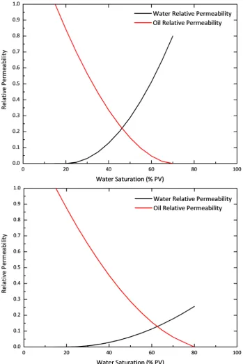
(14)

The relative permeability of each phase depends on the phase saturations but does not depend directly on fluid flow properties [63]. If only a single phase is present the relative permeability has no physical meaning, but in a multiphase sys-tem, the flow of one phase interferes with the others, hence this influence is taken into account in the Darcy equation (krj≤ 1). It is usual in multiphase systems to use

correlations of the relative permeabilities expressed as functions of the wetting phase saturation (Equation (15) and Figure 5),

( )

,

( )

.

rw rw w rnw rnw w

k =k S k =k S (15)

[image:12.595.196.546.72.596.2]

Figure 5. Relative permeability for oil-wet (left) and water-wet (right) formation rocks.

permeability, these depend on empirical constants (e.g., if the system is oil-wet or water-wet), so several models have been developed through the years [64]-[70].

2.3. Compositional Models

phases. This assumption is valid for two phase flows of water/brine and oil, which is often the case in primary and secondary recovery mechanisms. In EOR processes, mass transfer and compositional effects are deemed essential to model accurately as they may become the driving mechanisms for the displacing process. A typical re-servoir fluid may consist of several different chemical pseudo-components. Fully compositional models must be used when the fluid flow depends strongly on com-ponent transfer between phases. In fact, many EOR techniques, mainly chemical and miscible gas processes, are specifically designed to take advantage of the phase behavior of multicomponent fluid systems. Because these components may be transferred between phases (and change their composition), the basic conservation laws must be expressed for each component instead for each phase. For a chemical flooding compositional model, the governing differential equations consist of a mass conservation equation for each component, Equation (16), and Darcy’s law for each phase [20][71][72].

(

)

(

)

(

)

1

, 1, 2, , p

N

j j j j j j j

i i i i i i comp

j

z c u D c q Ad i N

t ρ φ = ρ t ρ φ

 

∂ _{= −∇ ⋅ − ∇ + −} ∂ ₌

 

∂ _

∑

_ ∂  (16)

1 1

, 1

p comp

N N

j j j

i i i

j i

z S c c

= =

=

∑

∑

= ₍₁₇₎

Here zi is the overall concentration of component i calculated by Equation (17), Ncomp is the number of components in the system, cij is the volumetric

concentra-tion of the component i in the phase j, j i

D is the diffusion-dispersion tensor of the

component i in the phase j, and Adi is the amount of component i adsorbed by the

rheological correlations (Power Law, Carreau-Yasuda, Unified Viscosity Model

[73]).

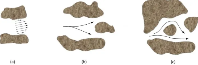
In addition to the advective, directional movement of a component described by the Darcy phase velocity, components may also move due to dispersive forces. The simplest movement is molecular diffusion described by the random Brownian mo-tion of molecules. Such momo-tion is usually considered in reservoir simulamo-tion of neg-ligible importance compared to other forces acting on the fluid. A more substantial phenomenon is mechanical dispersion. Narrow channel flows experience parabolic diffusion along the fronts (Taylor dispersion) and the irregular pore networks dis-perse the mass at a microscale (Figure 6). The tensor of hydrodynamic dispersion considering the mentioned effects is expressed in Equation (18) [20][39][46][47] [74],

( )

( )

2

j j j j j j j j

i i

D =φS dm I+ u _dl E u +dt E⊥ u _ (18)

where j i

dm denotes the molecular diffusion constant of the component i in the

phase j, the factors dlj and dtj are the parameters of longitudinal and transversal

dispersivity of the phase j, j ₂

u is the Euclidean norm of the phase velocity, and

( )

j

E u is the orthogonal projection along the velocity field as expressed in

Equa-tions (19) and (20). Mechanical dispersion models the spreading of the component on the macroscopic level due to the random structure of the porous medium and depends on the size and direction of the flow velocity.

( )

( )

( )

( )

( )

2

2 2

2 2

1

j j j j j

x x y x z

j j j j j j

y x y y z

j

j j j j j

z x z y z

u u u u u

E u u u u u u

u

u u u u u

 

 

 

= _{ }

 

 

 

(19)

( )

j

( )

j

E⊥ u = −I E u (20)

[image:14.595.199.547.532.647.2]

The dispersion part of the tensor is significantly larger than the molecular diffu-sion; also, dlj is usually considerably larger than dtj and their relationship can be

expressed as a function of the Peclet number [20] [46]. Nevertheless, at low Peclet numbers (Pe < 10) both dispersitivies are of the same order of magnitude [75]-[77]. Dispersion can represent small scale movements not captured by the REV used in the mathematical model, but according to Heimsund [28], taking this into account in the numerical model may be troublesome [78][79]. It is worth mentioning that some numerical schemes, especially first order methods (see point 3.2), add artifi-cial diffusion which is most of the times far greater than the physical dispersion discussed here. It is then advisable that when using naturally dissipative schemes the physical dispersion to be neglected [28][54][80].

If a compositional model is formed by a system of Ncomp components and Np

phases, there are a total of Np⋅

(

Ncomp +3

)

unknowns. The unknowns in each grid block are: Np⋅Ncomp concentrations, for each component on each phase, and 3Np

values for saturation, pressure and Darcy velocities. The governing system de-scribed previously include Ncomp conservation of mass equations, Np − 1 capillary

pressure relationships, Np Darcy equations, Np phase constraints, one saturation

constraint. To define the system of equations a number of Ncomp⋅

(

Np−1

)

extra relationships shall be defined so as to define the system, considering an isothermal medium and local thermodynamic equilibrium. This is usually determined by equi-librium thermodynamic considerations [20] [42] [81]-[83]. These relationships take the form of Equation (21) relating components i1 and i2 of phase j,

(

)

1

1 2 1 2 1 2 2

, , , , , .

j

i j j j

i i i i i i

j i

c

K T p p c c

c = (21)

2.4. Energy Equation

In case the flow cannot be considered isothermal, or the recovery process involves the addition of considerable amounts of energy to the reservoir, an extra condition and variable must be introduced to the system. The conservation of energy, Equa-tion (22), and its dependent variable, the temperature, are then added to the system. The major difference with respect to the other equations is that the energy is also conducted by the rock formation, and not only between the phases. If the local thermal equilibrium concept is applied, the temperature in the REV for all the phases and the porousmedium is considered to be the same and the energy equa-tion is as follows [20],

(

)

(

)

(

)

1 1

1

p p

N N

j j j j j j

s s t H L

j j

S U C T u H k T q q

t φ = ρ φ ρ = ρ

   

∂ _{+ − + ∇ ⋅ − ∇ = −}

   

∂ 

∑

 

∑

 (22)

where Uj is the specific internal energy, Csthe specific heat capacity of the rock, Hj

the enthalpy of the phase, kt the thermal conductivity tensor, qH the enthalpy

source term, and qL the heat loss. In most of the chemical EOR operations, the heat

transfer is considered negligible and therefore an isothermal assumption is valid.

2.5. Well Models

wells), open hole through which fluid can flow in and out of the reservoir, accord-ing to the strategies or its degree of maturity. These are cemented and then perfo-rated along specific intervals (multi-zone wells). The primary function of produc-tion wells is to extract hydrocarbons and later on, the water/chemical products in-jected as part of EOR processes. On the other hand, injection wells can be used for disposal of certain fluid (e.g. CO2 storage) as well as to inject chemical solutions so

as to increase the recovery efficiency, sweeping the oil towards production wells. These wells are controlled through surface facilities (e.g. choke valves, Christmas trees) (Figure 7).

The main purpose of a well model is to represent the flow in the wellbore and provide equations that serve as input for the mass conservation and Darcy equa-tions, to calculate the flow rate of each component being injected or produced. Generally, the bottomhole pressure is significantly different from the average pres-sure in the perforated grid blocks. Modeling injection and production of fluids us-ing point sources causes numerical problems in the flow field, so the concept of Productivity/Well Index (PI) was introduced in the form − =q PI p

(

−pwf

)

, to re-late the bottomhole pressure pwf to the numerically computed pressure p inside the

model [19]. The well index PI takes into account the geometric characteristics of the well and the properties of the surrounding rock, as it is indicated in Equation (23).

Peaceman [85] developed a numerical correlation to calculate the productivity index. Assuming steady-state radial flow, the well index for an anisotropic medium represented on a Cartesian grid in three dimensions yields,

1 2

1 2 1 2

2 2

0 1 4 1 4

0

2π

, 0.28

ln

y x

j _{y x}

x

j r

j

y x

w _{y x}

K K

y x

K K

K Ky z k

PI r

r _s K K

r _{K K}

µ

_{   } 

_{  ∆ +  ∆} 

 

_{   } 

∆ _{ }

= ⋅ =

  ₊     

  _{ }  _ _ + 

  _{   }

(23)

where s is the skin factor, rw is the well radius and r0 is the effective block radius at

which the steady-state pressure equals the computed block pressure. The Peaceman model has been also extended to horizontal wells and it was modified to take into account non-square grids, boundary blocks and non-Darcy effects [45] [86]-[89].

3. Numerical Techniques for Fluid Flow in Porous Media

[image:17.595.237.506.72.669.2]

Several numerical formulations are employed to solve the non-linear systems of equations. The most stable approach is a fully implicit solution technique in pres-sure and saturation/concentration, but this generally leads to large, ill-conditioned matrices. Another scheme broadly utilized in compositional formulation consists, in order to reduce the level of implicitness, to solve the pressure equation system implicitly (which can be viewed as an overall volume balance) plus a sequence of (Ncomp − 1) components conservation equations [20] [90]-[95]. The conservation

equations have a strongly hyperbolic character due to the advective term. The over-all technique is cover-alled an IMPEC (implicit in pressure, explicit in concentration). IMPEC methods are often limited by stability restrictions on the time step size due to their explicit scheme, but solutions do not suffer less smoothing than fully impli-cit methods, which strongly affect the performance prediction of compositional models [72]. Different implicit techniques are also used and often provide en-hanced efficiency, allowing bigger time steps than those employed with IMPEC. One of these methods is the implicit pressure and saturation (IMPSAT) procedure, in which pressures and (Np − 1) saturations (but not compositions) are determined

implicitly [82]. Different techniques worth of mentioning are: Adaptive implicit (AIM) [82][96], bilinear approximation techniques [97], preconditioning schemes

[98] [99], parallel computing and adaptive mesh refinement (AMR) in composi-tional simulation [72][100][101].

3.1. Numerical Schemes

The aim of this section is the derivation and explanation of the numerical schemes to be used for solving differential equations presented above, as well as also explain the reasons for the occurrence and possible numerical solutions of certain pheno-mena that affect simulation results [102]. The equation to be used as a model is the one-dimensional advection-diffusion Equation (24), which is a simplification of the continuity equation presented for the compositional model,

2 2.

u u u

v D

t x x

∂ ₊ ∂ ₌ ∂

∂ ∂ ∂ (24)

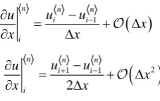
Using a finite-difference approach the continuous domain is transformed into a discrete representation with a finite number of points in both a spatial (i) and tem-poral ( n ) grids. Then, the time derivative in previous equation is expressed using

a Taylor series expansion around the point n i

u yielding Equations (25) and (26),

( )

2 2

1 3

2

2

n n

n n

i i

i i

u t u

u u t t

t t

+ _{= + ∆} ∂ ₊∆ ∂ _{+ ∆}

∂ ∂  (25)

( )

1

n n n

i i

i

u u

u

t

t t

+ ₋

∂ _{= + ∆}

∂ ∆  (26)

where 

( )

∆t is the Bachmann-Landau notation used to describe the extra error

this case the overall order of the equation is determined by the differential operator with the largest truncation error. Noteworthy is also that while the truncation error is expressed for the differential operator, the numerical algorithms will not be ex-pressed in terms of the differential operators and will therefore have different (usually smaller) truncation errors. Following a similar procedure, the finite-dif- ference approximations in Equations (27) and (28) are obtained for the space de-rivative in backwards and centered forms as,

( )

1

n n n

i i i u u u x x x − − ∂ _{= + ∆}

∂ ∆  (27)

( )

2

1 1 _.

2

n n n

i i i u u u x x x + − − ∂ _{= + ∆}

∂ ∆  (28)

Even though the centered scheme has a higher order of precision, it generates unstable results when applied to the advection equation (wave transport equation). Hence, numerical methods using only points that are “upwind” of the wavefront are employed [103].

The inclusion of diffusion phenomena in the description of a fluid flow leads to non-trivial complications in the numerical solution of the mass conservation equa-tions. From an analytical point of view, the resulting equations are no longer purely hyperbolic PDE’s but rather mixed hyperbolic-parabolic PDE’s. This means that the numerical method used to solve them must necessarily be able to cope with the parabolic part of the equations. For the diffusive term, the second order derivative is usually discretized using a centered scheme yielding Equation (29),

( )

2 2 1 1 2 2 2 .

n _{n n n}

i i i

i

u u u

u x x x + − + − ∂ = + ∆

∂ ∆  (29)

The final upwind discretized equation (FTUS-Forward in Time, Upwind in Space) and its matrix form for the advective-diffusive system are then presented in Equations (30) and (31), respectively.

(

)

1

1 1 1

2

2

,

n n n n n n n

i i i i i i i

u u u u u u u

v D x t

t x x

+

− + −

− − − +

+ = + ∆ ∆

∆ ∆ ∆  (30)

1

n n

Au + =Bu +C (31)

In Equation (30) the order of accuracy is expressed as function of both indepen-dent variables 

(

∆ ∆x, t

)

, inferring that both discretization schemes for spatial and

temporal grids have influence in the total error of the numerical model. The solu-tion at the new time-step n+1 can be calculated explicitly from the quantities

that are already known at the previous step n . This differs with an implicit

scheme in which the finite-difference representations of the differential equation are expressed of terms at the new time-level n+1 . These methods require solving

[image:19.595.316.430.178.250.2]

a number of coupled algebraic equations.

[image:20.595.198.551.87.421.2]

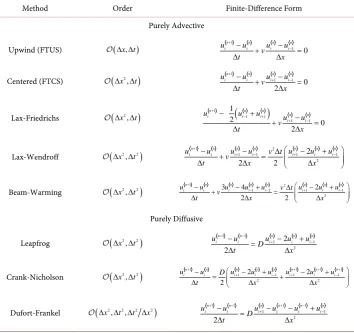
Table 1. Most common numerical schemes used in reservoir simulation.

Method Order Finite-Difference Form

Purely Advective Upwind (FTUS) (∆ ∆x, t)

1

1

0

n n n n

i i i i

u u u u v t x + − − ₊ − ₌ ∆ ∆

Centered (FTCS)

(

2

)

,

x t

∆ ∆



1

1 1 ₀

2

n n n n

i i i i

u u u u v t x + + − − − + = ∆ ∆

Lax-Friedrichs

(

2

)

,

x t

∆ ∆

 1

(

1 1

)

1 1

1

2 ₀

2

n n n

n n i i i

i i

u u u _{u u}

v t x + − + + − − + ₋ + = ∆ ∆

Lax-Wendroff

(

2 2

)

,

x t

∆ ∆



1 2

1 1 1 1

2

2

2 2

n n n n n n n

i i i i i i i

u u u u v t u u u v

t x x

+ + −  + −  − ₊ − ₌ ∆ − +     ∆ ∆ _ ∆ _

Beam-Warming

(

2 2

)

,

x t

∆ ∆



1 2

1 2 1 1

2

3 4 2

2 2

n n n n n n n n i i i i i i i i

u u u u u v t u u u

v

t x x

+ − −  + −  − ₊ − + ₌ ∆ − +     ∆ ∆ _ ∆ _ Purely Diffusive

Leapfrog

(

2 2

)

, x t ∆ ∆  1 1 1 1 2 2 2

n n n n n

i i i i i

u u u u u

D t x + − + − − − + = ∆ ∆

Crank-Nicholson

(

2 2

)

,

x t

∆ ∆



1 1 1 1

1 1 1 1

2 2

2 2

2

n n n n n n n n i i i i i i i i

u u D u u u u u u

t x x

+ + + + + − + −   − − + − + = _ + _ ∆ _ ∆ ∆ _

Dufort-Frankel

(

2 2 2 2

)

, ,

x t t x

∆ ∆ ∆ ∆



1 1 1 1

1 1

2

2

n n n n n n

i i i i i i

u u u u u u

D t x + − + − + − − ₌ − − + ∆ ∆

advective or diffusive 1D equation.

Table 2 summarizes the most common discretization schemes and their orders of accuracy [102]. Higher orders schemes allow increasing the accuracy of the numer-ical model but at the cost of requiring a higher number of points to make the eval-uation of the derivatives. This increases both the computational cost and the diffi-culty of evaluating derivatives near the boundaries.

A key factor in all numerical schemes is the issue of how treating the solution on the boundaries of the spatial grid as the time evolution proceeds. Two types of con-ditions are generally used in reservoir simulation to describe whether the Darcy velocity or the pressure of a phase at the boundaries. These are: Dirichlet type con-ditions, when the values of the relevant quantity are imposed at the boundaries of the grid (these values can be either functions of time or be held constant), and Von Neumann type conditions, when the values of the derivatives of the relevant quan-tity are imposed.

3.2. Numerical Dissipation and Dispersion

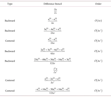
[image:20.595.196.551.90.423.2]

[image:21.595.195.551.86.396.2]

Table 2. Higher order schemes for first and second order derivatives.

Type Difference Stencil Order

u x

∂ ∂

Backward 1

n n i i u u x − −

∆ ( )∆x

Backward 3 4 1 2

2

n n n

i i i

u u u x − − − + ∆

( )

2 x ∆ 

Centered 1 1

2 n n i i u u x + − − ∆

( )

2 x ∆ 

Backward 2 1 3 6 1 2

6

n n n n

i i i i

u u u u x + + − − + − ∆

( )

3 x ∆ 

Backward 25 48 1 36 2 16 3 3 4

12

n n n n n

i i i i i

u u u u u

x − − − − − + − + ∆

( )

4 x ∆  2 2 u x ∂ ∂

Centered 1 1

2

2

n n n

i i i

u u u x + − + − ∆

( )

2 x ∆ 

Centered 2 1 1 2

2

16 30 16

12

n n n n n

i i i i i

u u u u u

x + + − − − + − + − ∆

( )

4 x ∆ 

the numerical scheme. The LTE can be expressed as a function of higher order de-rivatives [104][105],

Original PDE Modified Equation

2 2 0

u u u

v D t x x

∂ ₊ ∂ ₋ ∂ ₌

∂ ∂ ∂

2 2 2 1

2 2 1

2 2 2 1

1 1

n n

n n n n

n n

u u u u u

v D a a

t x x x x

+ ∞ ∞ + + = = ∂ ₊ ∂ ₋ ∂ ₌ ∂ ₊ ∂ ∂ ∂ ∂

∑

∂

∑

∂

The procedure to calculate this error and assess its contribution to the numeric solution is straight-forward. It consists in performing an expansion in a double Taylor series around a single point n

i

u , both in spatial and temporal grids to obtain

a modified PDE. Besides, the high-order time derivatives as well as mixed deriva-tives must be transformed in terms of space derivaderiva-tives using this modified PDE. The analysis for the truncation error in the 1D advective-diffusive equation is pre-sented using two numerical schemes: firstly the upwind scheme and subsequently the Lax-Wendroff scheme. For the upwind scheme it yields Equation (32),

(

)

1

1 1 1

2

2

,

n n n n n n n

i i i i i i i

u u u u u u u

v D x t

t x x

+

− + −

− ₊ − ₌ − + _{+ ∆ ∆}

∆ ∆ ∆  (32)

( )

2 2 3 3

1 4 2 3 2 6 n n n n n i i

i i i

u t u t u

u u t t

t t t

+ _{= + ∆} ∂ ₊∆ ∂ ₊∆ ∂ _{+ ∆}

( )

2 2 3 3 4 4

5

1 2 3 4

2 6 24

n n n

n

n n

i i

i _{i i i}

u x u x u x u

u u x x

x x x x

+ = + ∆ _∂∂ +∆ ∂_∂ +∆ ∂_∂ +∆ ∂_∂ + ∆ (34)

( )

2 2 3 3 4 4

5

1 2 3 4

2 6 24

n n n

n

n n

i i

i _{i i i}

u x u x u x u

u u x x

x x x x

−

∂ ∆ ∂ ∆ ∂ ∆ ∂

= − ∆ + − + + ∆

∂ ∂ ∂ ∂  (35)

Introducing these terms from Equations (33), (34) and (35) in the numerical scheme presented in Equation (32) it yields,

(

)

2 2 3 2 2 3 3 4 4

2 3 2 3 4

2 2 4

2 4 3

2 2 4

2 6 2 6 24

, 12 n n i i n i

u t u t u v u x u x u x u

x

t t t x x x x x

D u x u

x x t

x x x

∂ ₊∆ ∂ ₊∆ ∂  ₊ _∆ ∂ ₋∆ ∂ ₊∆ ∂ ₋∆ ∂  _{∂ ∂ ∂}  _∆  _{∂ ∂ ∂ ∂}       ∂ ∆ ∂  = _∆ + _ + ∆ ∆ ∆ _ ∂ ∂ _  (36)

Rearranging Equation (36) to split the original PDE and the truncation error,

(

)

2 2

2 2 3 2 2 3

2 3 2 3

3 4 2 4

3 3

4 4

2 6 2 6

,

24 12

n

n n

i i i

n n n n

i i i i

n n

i i

u u u

v D

t x x

t u t u v x u v x u

t t x x

v x u D x u

x t x x ∂ ₊ ∂ ₋ ∂ ∂ ∂ ∂ ∆ ∂ ∆ ∂ ∆ ∂ ∆ ∂ = − − + − − ∂ ∂ ∂ ∂ ∆ ∂ ∆ ∂ + + + ∆ ∆ ∂ ∂   (37)

Now the temporal derivatives in Equation (37) are transformed in space deriva-tives. Furthermore, using Courant and Peclet dimensionless groups presented in Equation (38) the LTE for the method is derived in Equation (39),

,

v t xv

Cr Pe

x D

∆ ∆

= =

∆ (38)

(

)

(

)

2 2

2 2

2 3

2 3 3

3

1 2 6

3 2 1 ,

6

n n

n n

i i i i

n

i

u u u v x u

v D Cr

t x x x

v x Cr u

Cr Cr x t

Pe x ∂ ∂ ∂ ∆ ∂ + − = − − + ∂ ∂ ∂ ∂ ∆  ∂ + _ − − + _{ ∂} + ∆ ∆     (39)

The numerical scheme does not solve the original PDE, but a modified PDE with extra terms of higher order derivatives. The extra term containing the second order derivative is interpreted as a numerical diffusion, additional to the physical coeffi-cient D. As long as the Cr < 1 condition is met, the numerical solution will produce an artificial smearing given by the term

(

v x∆ 2 (1

)

−Cr). The term containing the

[image:23.595.197.549.71.611.2]

Figure 8. Influence of even (left) and odd (right) higher order derivatives in the numerical solution (adapted from [104]).

counteract the added terms by the numerical scheme; the non-oscillatory shock- capturing methods, TVD (Total Variation Diminishing) or flux-limiters [19] can also be listed as improved schemes to overcome these effects. To reduce the influ-ence of these differinflu-ences a possible solution is also to use schemes of superior or-ders (see Table 2). As an example of these techniques, the same analysis done for the upwind scheme is performed using the Lax-Wendroff method. The latter due to the fact that the time derivative is expressed as a second order Taylor series expan-sion [104][105]. The numerical model to solve is presented in Equation (40),

(

)

1 2

2 2

1 1 1 1

2

2

, .

2 2

n n n n n n n

i i i i i i i

u u u u v t u u u

v D x t

t x x

+

+ −   + −

− − ∆ − +

+ =_ + _ + ∆ ∆

∆ ∆ _{ } ∆  (40)

Following a procedure similar to the previous scheme it renders Equation (41),

(

)

2 2 3

2 3 3

2 3

6

1 , .

6

n n

n n

i i i i

u u u v x Cr u

v D Cr x t

t x x Pe x

∂ ₊ ∂ ₋ ∂ _{= −} ∆  _{− +} ∂ _{+ ∆ ∆}

 

∂ ∂ ∂  ∂  (41)

As shown, the first diffusive term in the LTE has disappeared leaving the disper-sive term as the main source of error in this method. Since this term is negative, the spurious oscillations occur behind steep fronts. It is worth mentioning that a more accurate numerical scheme is not necessarily a preferable one. As an example, the upwind and the Lax-Friedrichs methods are both dissipative, thelatterisgenerical-lymoredissipativedespitebeingofhigherorderaccuracyinspace.

3.3. Flux Limiters

In the previous section two of the most common numerical schemes utilized were introduced, and the advantages or disadvantages of each were studied and inferred. While the upwind scheme can handle steep gradients, it is very diffusive and moreover a first order scheme; on the other hand, Lax-Wendroff is a second order scheme, less diffusive but presents serious problems when sharp gradients are present in the system. Therefore, new numerical schemes were published coupling low- and high-resolution methods, taking advantage of the mentioned characteris-tics [104][106]-[115]. For this analysis, it is considered the 1D advection-diffusion Equation (42) in term of fluxes, with no diffusive terms.

(

)

1

1 2 1 2

1

0.

n n

n n

i i

i i

u u

F F

t x

+

+ −

−

+ − =

∆ ∆ (42)

The idea behind this concept is then to write the fluxes as a function of low- and high-resolution numerical schemes as in Equation (43), using a proportionality factor.

( )

( )

1 2 1 2 1 2 1 1 2 1 2

n high low

i i i i i i i

F± =ψ± r ⋅F± + − ψ± r ⋅F± (43)

1 1 . i i i i i u u r u u − + − =

− (44)

Using the FTUS and Lax-Wendroff in Equation (45) as low- and high-resolution schemes respectively, the flux is calculated according to Equation (46),

(

)

₍

₎

1 2 1 2 1

1 ,

2

low high

i i i i i i

v Cr

F₊ = ⋅v u F₊ = ⋅ +v u − u₊ −u (45)

( )

(

)

(

)

1 2 1

1 2

1

. 2

n

i i i i i

i

v Cr

F+ v u

ψ

+ r u+ u

−

= ⋅ + ⋅ − (46)

Finally, the discretized advection Equation (47) is written in terms of the flux li-miter parameter,

(

)

_{( )}

₍

₎

(

)

_{( )}

₍

₎

1

1 2 1

1 2 1

1 2 1

2

n n n n

i i i i i i

n n

i i i i

Cr Cr

u u Cr r u u

Cr Cr

r u u

ψ ψ + − − + + −   = −_ − _ − −   − − −  (47)

(

)

_{( ) (}

)

1 2

( )

₍

₎

1

1 2 1

1 2

1 1

1 .

2 2

i i

n n n n

i i i i i i

i

r

Cr Cr

u u Cr r u u

r ψ ψ + + − − +  − −  = −  − +  −  

  (48)

Equation (48) resembles the FTUS scheme with a modified Courant number

[107][110][111]. The properties of stability and monotony of the FTUS are well- known. So for the new numerical scheme to meet these requirements the In Equa-tion (49) must be valid,

(

)

_{( ) (}

)

1 2

( )

1 2

1 2

1 1

0 1 1.

2 2 i i i i i r Cr Cr Cr r r ψ ψ + − +  − −  ≤  − + ≤  

  (49)

This is valid for positives values of r, when the following two conditions in In Equation (50) are met (Figure 9).

( ) ( )

0 r , r 2

r

ψ ψ

 

≤ ≤

  (50)

Further, more restrictive constraints are applied in order to make the scheme second order in accuracy (Figure 10). Several high-order flux limiter functions were developed within this region. These are characterized by a low numerical disper-sion in high gradient fields as well as being less diffusive than traditional schemes (FTUS) in low gradient advection phenomena (Table 3 and Figure 11).

3.4. Consistency and Stability

This review concludes with the study of three concepts related with numerical si-mulation. The first to be defined is the consistency of a numerical scheme: Given a PDE in its operator form 

( )

u − =f 0, a finite difference scheme applied to this

PDE

( )

n n 0

(

p, p

)

i i

u f x t

∆ − = + ∆ ∆

  , and the LTE being expressed by means of a representative variable

( )

p

( )

p ,

h Ch h C

[image:26.595.229.523.73.300.2]

Figure 9. Total variation diminishing (TVD) region for the flux limiter func-tion.

Figure 10. Total variation diminishing second-order accuracy region for the flux limiter function.

[image:26.595.231.521.351.580.2]

[image:27.595.198.547.71.247.2]

Figure 11. Second-order TVD functions presented in Table 3.

Table 3. Most commonly used flux limiter functions.

Type Flux Limiter Function Reference

Superbee max 0, min 2 ,1 , min_ ( r ) ( )r, 2_ Roe [116]

Minmod max 0, min_ ( )r,1_ Roe [117]

Van Leer

1

r r

r

+

+ Van Leer [118]

Van Albada ₁ 22

r r r

+

+ Van Albada [119]

Koren max 0, min 2 ,2 , 2 3

r r

  + 

 

 _{ }

  Koren [120]

CHARM ₍( ₎2)

3 1

1

r r

r

⋅ +

+ Zhou [121]

MUSCL max 0, min 2 ,1 , 2 2

r r

  + 

 

 _{ }

  Van Leer [122]

can grow boundless, amplifying the errors until the system eventually collapses. This is ensured introducing the concept of numerical stability. To understand this, a system of equations written in the form of modified PDE Equation (31) is analyzed. Perturbations at the baseline as well as at a generic time n = ∆m t due

to numerical errors during the simulation are introduced. This is expressed as

n n n

i i i

u =u + and u_i0 =u_i0 +_i0 . Replacing these values it renders Equation

(51),

1 1 1

.

n n n n n n

Au + =Bu →A + =B → + =G (51)

where G is the amplification matrix of the numerical perturbations in the system.

[image:27.595.192.553.298.530.2]

with the initial perturbation can be established.

1 2 1 0

n n n n

G G G

+ _{= =} − _{= =}



    (52)

Equation (52) exposes a central issue in the stability analysis: the question of whether amplification matrices have their powers uniformly bounded. In order for the numerical errors to not be amplified during the simulation, a stability restric-tion is then defined Gn ₂≤K K, ∈. According to this condition, the only way to keep the errors limited and prevent their propagation and amplification is fulfilling the condition established in Equation (53), ensuring the existence of K.

( )

2 , 1

n

G ≤K n→ ∞ ⇔ρ G ≤ (53)

where ρ

( )

G is the spectral radius of the amplification matrix. Hence, a one-step

finite difference scheme approximating a PDE is a convergent scheme if and only if it renders the exact solution of the original PDE, expressed mathematically in Equ-ation (54),

( )

0

0 0

lim , _{n x}m t 0, , , .

x t

u x t u_∆∆ m n + x n x t m t

∆ → ∆ →

 ₋ _{= ∀ ∈ ∧ = ∆ = ∆}

   (54)

[image:28.595.196.548.430.685.2]

These three concepts can be summarized in the following theorem: Given a properly posed initial-value problem and a finite difference approximation to it, that satisfies the consistency criterion, stability is the necessary and sufficient con-dition for convergence. This theorem, known as the “Lax-Richtmyer equivalence theorem” or Fundamental Theorem of Numerical Analysis (Figure 12), is quite important since it shows that consistency, stability and convergence are strictly