Feedback Chaotic Synchronization with Disturbances

(1)

http://www.scirp.org/journal/ijmnta ISSN Online: 2167-9487

ISSN Print: 2167-9479

Feedback Chaotic Synchronization with

Disturbances

Mingjun Wang, Wanbo Yu, Jing Zhao

School of Information Engineering, Dalian University, Dalian, China

Abstract

Based on Lyapunov stability theorem, a method is proposed for feedback synchronization with parameters perturbation and external disturbances. It is proved theoretically that if the perturbation and disturbances are bounded, the synchronization error can be ensured to approach to and stay within the pre-specified bound which can be arbitrarily small. Some typical chaotic sys-tems with different types of nonlinearity, such as Lorenz system and the orig-inal Chua’s circuit, are used for detailed description. The simulation results show the feasibility of the method.

Keywords

Lyapunov Stability Theorem, Feedback Synchronization, Parameters Perturbation, External Disturbances, Robustness

1. Introduction

In 1990, Pecora and Carroll presented the conception of “chaotic synchroniza-tion” and introduced a method to synchronize two identical chaotic systems with different initial conditions [1] [2]. Since chaos control and synchronization have great potential applications in many areas such as information science, medicine, biology and engineering, they have received a great deal of attention. Numerous researches have been done theoretically and experimentally [3] [4] [5]. Muradi and Kapitaniak expanded Corroll and Pecora’s work, presented a single unidirectional coupled synchronization scheme [6] [7]. Celka achieved chaos synchronization by using the time-delay feedback method [8]. Agiza et al.

synchronized Rössler and Chen systems via active control method [9] and Im-pulsive control [10]. Guo et al. proposed a simple adaptive-feedback controller for chaos synchronization [11]. Agrawal et al. realized the synchronization of fractional order chaotic systems using active control method [12]. Norelys et al. How to cite this paper: Wang, M.J., Yu,

W.B. and Zhao, J. (2017) Feedback Chaotic Synchronization with Disturbances. Inter-national Journal of Modern Nonlinear Theo- ry and Application, 6, 1-10.

https://doi.org/10.4236/ijmnta.2017.61001

Received: September 20, 2016 Accepted: January 8, 2017 Published: January 11, 2017

http://creativecommons.org/licenses/by/4.0/

(2)

presented the adaptive synchronization of fractional Lorenz systems using a re-duced number of control signals and parameters [13]. Kajbaf et al. used sliding mode controller to obtain chaotic systems [14]. Wang et al. proposed a new feedback synchronization criterion based on the largest Lyapunov exponent [15]. However, most synchronization criterions were obtained under ideal cir-cumstances. If parameters perturbation and external disturbance exist, this kind of criterions will take no effect. According to this practical problem, some solu-tions have been presented. For examples, Jiang et al. proposed a LMI criterion [16] for chaotic feedback synchronization. Although the simulations showed that it is robust to a random noise with zero mean, but no rigorous mathematical proof was provided and we can’t determine if their method is effective for other kinds of noise. In Ref. [17], parameters perturbation was involved in their scheme. The theoretical proof and numerical simulations were given in their work, but external disturbance didn’t receive attention, which made their method unila- teral.

Above all, these methods are effective, but still lack generality or robustness. In this paper, we propose a practical synchronization scheme for chaotic syn-chronization with parameters perturbation and external disturbance. Rigorous mathematical proof is provided, and simulation results show the feasibility and robustness of our scheme.

2. Theory and Method

In the following scheme, a universal robust synchronization method is proposed. In the method, synchronization will be achieved with bounded parameter dis-turbances and noise.

Suppose a class of ideal chaotic systems as

( )

f

= +

X AX X

where AX is the linear part, f X

( )

is the nonlinear part, then the system can be described as

( )

(

t

)

f

( )

f

(

,t

)

( )

t

= ∆ + + ∆ +

X A + A X X X D (1)

where ∆A

( )

t and ∆f

(

X,t

)

are the parameters perturbation, D

( )

t is the external disturbance. Choose system (1) as the drive system, the relevant re-sponse system can be described as

( )

(

′ t

)

f

( )

f′

( )

,t

(

)

′

( )

t

= ∆ + + ∆ − − +

Y A + A Y Y Y K Y X D (2)

where ∆A′

( )

t , ∆f′

( )

Y,t and D′

( )

t are the relevant disturbances in the re-sponse system. We choose K=diag k k

(

1, 2,,kn

)

(n is the dimension of the chaotic system). Let the error vector E=Y−X, then the error is

(

)

( )

,

(

,

)

( )

f f t t

f t f t t t

′

= − + − + ∆ − ∆

′ ′

+ ∆ − ∆ + −

E A K E Y X A Y A X

Y X D D



(3)

Set a pre-defined bound ε_{for the synchronization error, suppose}

[

]

T

1, 2, , n

e e e

=

E  , choose suitable K to ensure lim _i

( )

(3)

(

i=1, 2,,n−1,n

)

, then system (1) and system (2) achieve approximate syn-chronization, the precision is ε_{. When}ε _{is very small, we can consider} sys-tem (1) and syssys-tem (2) have been synchronized.

Choose the following Lyapunov function 2 1 1 2 n i i V e =

=

∑

_{, yield}

1

n

i i i

V e e

=

∑

 _ _.

According to Equation (3), the derivative of ej can be described as

(

)

(

)

1 1

, ,

n n

j ji i ji i j j j j

i i

e a e h e g d k e

= =

=

∑

+

∑

X Y + X Y + −

 (4)

ji

a is the element of matrix A, hji

(

X Y,

)

and gj

(

X Y,

)

is bounded, dj

is bounded external disturbances, kj is feedback coefficients．When the errors go

beyond ε _{, we have}

(

)

₂ ₂

₍

₂ ₂

₎

(

)

₍

₂ ₂

₎

1 1

, ,

2 2

n n

j j ji ji

j j j j j i j i j

i i

g d a h

e e e k e e e e e

ε = =

+

≤ X Y − +

∑

+ +

∑

X Y +

 (5)

(

)

₍

₎

(

)

₍

₎

(

)

(

)

1

2 2 2 2 2 2

1 1 1

2

1 1 1 1 1

, ,

2 2

, , ( , )

.

2 2 2 2

n

j j j

n n n

j j ji ji

j j j i j i j

j i i

n n n n n

j j ji ij ji i j

j j

j i i i i

V e e

g d a h

e k e e e e e

g d a a h h

k e ε ε = = = = = = = = = =  +    ≤ − + + + +      +    = − + + + +    

∑

X Y X Y

X Y X Y X Y

 _

(6)

If

(

)

(

)

(

)

1 1 1 1

, , ,

2 2 2 2

n n n n

j j ji ij ji ji

j

i i i i

g d a a h h

k

ε = = = =

+

> X Y +

∑

+

∑

+

∑

X Y +

∑

X Y (7)

we can obtain

1

0

n

i i i

V e e

=

∑

<

 _ ₍₈₎

That is to say, when the error is not within the bound ε, it will exponentially converge to zero. Hence system (1) and system (2) will achieve approximate synchronization, the precision is ε_{at least.}

3. Numerical Simulations

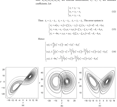
Lorenz system and the original Chua’s circuit have different types of nonlineari-ty. Next we will adopt the two systems for detailed description.

3.1. Taking Lorenz System as Example

Lorenz system [18] is described as

(

)

x a y x

y cx y xz

z xy bz

= −   ₌ _{− −}   = −     (9)

(4)

Figure 1. Obviously we have x ≤20, y ≤30, z ≤50.

Choose the following Lorenz system with parameters perturbation and exter-nal disturbances

(

)(

)

(

)

(

)

1 2 1 1

2 1 2 1 3 2 3 1 2 3 3

a

c

b

x a x x d

x c x x x x d

x x x b x d

ξ ξ ξ  = + − +  = + − − +   = − + +     (10)

as drive system, then the relevant response system is

(

)(

)

(

)

(

)

(

)

(

)

(

)

1 2 1 1 1 1 1 2 1 2 1 3 2 2 2 2 3 1 2 3 3 3 3 3

a

c

b

y a y y d k y x

y c y y y y d k y x

y y y b y d k y x

ξ ξ ξ ′ ′  = + − + − −  ′ ′ = + − − + − −   ₌ _{− +} _′ ₊ _′₋ ₋     (11)

In system (10) and system (11), ξ ξ ξ ξ ξ ξa, b, c, a′ ′ ′, b, c are parameters perturba-tion, d d d d d d1, 2, 3, 1′ ′ ′, 2, 3 are external disturbances, k1, k2, k3 are feedback

coefficients. Let

1 1 1 2 2 2 3 3 3

e y x

= −   = −   = −  (12)

Then e1=y1−x1, e2=y2−x2, e3 =y3−x3. The error system is

(

)

(

)

(

)

(

)

(

)

1 2 1 2 1 2 1 1 1 1 1 2 1 2 3 1 1 3 1 1 2 1 2 2 3 3 2 1 1 2 3 3 3 3 3 3

a a

c c

b b

e a e e y y x x d d k e

e ce e y e x e y x d d k e

e be y e x e y x d d k e

ξ ξ ξ ξ ξ ξ ′ ′  = − + − − − + − −  ′ ′ = − − + + − + − −   _{= −} ₊ ₊ ₋ _′ ₋ ₊ _′₋ ₋     (13) Hence

(

)

(

)

(

)

(

)

(

)

(

)

2 2 2 2 2 1 1 1 2 1 1 1 1 1

3 1

2 2 2 2 2 2 2 2 2

2 2 1 2 2 1 2 2 3 2 2 2 2

2 1

2 2 2 2 2 2 2

3 3 3 2 3 2 3 3 3 3 3

2

2 2 2

2 2

a

e e e e ae l e k e

y x

c

e e e e e e e e e l e k e

y x

e e be e e e e l e k e

[image:4.595.59.543.276.719.2]

 _≤ ₊ ₋ ₊ ₋    _≤ ₊ _{− +} ₊ ₊ ₊ ₊ ₋    ≤ − + + + + + −      (14)

(5)

where

(

2 1

)

(

2 1

)

1 1

1

1 1 2 1

2

3 3 3 3

3

a a

c c

b b

y y x x d d

l

y x d d

l

y x d d

l ξ ξ ε ξ ξ ε ξ ξ ε  ′ + + + + ′+ =    ′ + + ′ +  =    ′ + + ′ + =   (15)

Choose Lyapunov function

( )

(

2 2 2

)

1 2 3

1 2

V t = e +e +e (16) We have

( )

1 1 2 2 3 3

V t =e e +e e +e e (17) Substitute Equation (14) into Equation (17), obtain

3 2 2 3 2

1 1 1 2 1 2 2

2 2

3 1 3 3

1

2 2

. 2

c a y y a c y

V l k e l x k e

y

l b x k e

 − + +   + +  = + −  + − + + −        +_ − + + − _    If 3 2 1 1 3

2 2 1

2

3 3 1

2

1 2

2

c a y y

k l

a c y

k l x

y

k l b x

 − + +

> +  

 + +

 > − + + 

 

> − + + 



(18)

is satisfied, we will obtain V t

( )

<0. According to Lyapunov stability theorem,

the error system (13) will converge to zero when the error is not within the bound ε_,_i.e._{system (10) and system (11) will achieve approximate} synchroni-zation, the precision is ε_{at least}．

When the parameters perturbation and external disturbances are small, we can consider the variables of system (10) and system (11) are bounded as shown in Figure 1. Suppose the upper bounds of these disturbances and per-turbation are 0.5, choose ε =0.1, substitute Equation (15) into Equation (18), after calculating we obtain if

1 2 3 559 273 543 k k k >   >   >  (19)

is satisfied, Equation (18) will be always true.

In the simulation, suppose

ξ

a =0.5sin 2

( )

t ,

ξ

b=0.5 cos

( )

t ,

(

)

0.5 cos 1

c t

ξ

= + _,

ξ

a′ =0.5 cos 3

(

t+2

)

,

ξ

b′ =0.5sin 5

( )

t ,

ξ

c′ =0.5sin 2

( )

t ,

1, 2, 3, 1, 2, 3

(6)

and Equation (11). Let k1=560, k2=280, k3=550, Figure 2 shows the

his-tory of e t1

( )

, e t2

( )

, e t3

( )

in the error system (13) within 0.1 sec. From

Fig-ure 2, we can see that e t1

( )

, e t2

( )

, e t3

( )

are steady near zero at last.

3.2. Taking the Original Chua’s Circuit as Example

The original Chua’s circuit [19] is described as

( )

(

)

x a y x f x

y x y z

z by

 = − −

 _{= − +} 

 = − 

  

(20)

where f x

( )

=dx+0.5

(

c−d

)

(

x+ − −1 x 1

)

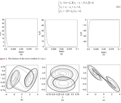
. In this paper choose a=9.78, 14.97

b= , c= −1.31 and d = −0.75 so that system (20) exhibits a chaotic be- havior [19]. The projections of the original Chua’s circuit’s attractor are shown in Figure 3. Obviously we have x ≤4, y ≤1,z ≤5.5.

Choose the following Chua’s circuit with parameters perturbation and exter-nal disturbances

(

)

(

( )

)

(

)

1 2 1 1 1

2 1 2 3 2

3 2 3

a

b

x a x x f x d

x x x x d

x b x d

ξ

 = + − − +

 _{= −} ₊ ₊



 = − + +

   

(21)

[image:6.595.62.541.317.725.2]

Figure 2. The history of the error (within 0.1 sec.).

(7)

As drive system, where

( ) (

1 d

)

1 0.5

(

c

) (

d

)

)(

1 1 1 1

)

f x = d+ξ x + c+ξ − d+ξ x + − x − , then relevant response system is

(

)

(

( )

)

(

)

(

)

(

)

(

)

1 2 1 1 1 1 1 1

2 1 2 3 2 2 2 2

3 2 3 3 3 3

a

b

y a y y f y d k y x

y y y y d k y x

y b y d k y x

ξ ξ  = + ′ − − + ′− −  ₌ ₋ ₊ ₊ _′₋ ₋   _{= − +} _′ ₊ _′₋ ₋     (22)

where f y

( ) (

1 = d+ξd′

)

y1+0.5

(

c+ξc′

) (

− d+ξd′

)

)(

y1+ −1 y1−1

)

. In system (21) and system (22), ξ ξ ξ ξ ξ ξ ξ ξa, b, c, d, a′ ′ ′ ′, b, c, d are parameters perturbation,

1, 2, 3, 1, 2, 3

d d d d d d′ ′ ′ are external disturbances, k1, k2, k3 are feedback

coeffi-cients. Let

1 1 1 2 2 2 3 3 3

e y x

= −   = −   = −  (23)

Then e1=y1−x1, e2=y2−x2, e3 =y3−x3. The error system is

( )

(

)

(

)

(

( )

)

(

( )

)

(

)

1 2 1 1 1 2 1 1 2 1 1 1 1 1 1

2 1 2 3 2 1 2 2

3 2 2 2 3 3 3 3

a a

b b

e a e e f y f x y y f y x x f x d d k e

e e e e d d k e

e be y x d d k e

ξ ξ ξ ξ  = − − − + ′ − − − − − + − −′  _{= − + +} _′_{− −}   _{= −} ₋ _′ ₋ ₊ _′₋ ₋     (24)

when the parameters perturbation and external disturbances are small, we can consider the variables of system (21) and system (22) are bounded as shown in Figure 4. Next we will substitute x ≤4, y ≤1,z ≤5.5 directly to simplify the

results, so we have

( )

{

1

}

(

)

(

)

sup f x ≤4 d +ξd + +c ξc + d +ξd =5 d +ξd + +c ξc (25)

( )

{

1

}

(

)

(

)

sup f y ≤4 d +ξ_d′ + +c ξ_c′+ d +ξ_d′ =5 d +ξ_d′ + +c ξ_c′ (26) Because

(

) (

)

(

) (

)

1 1 1 1 1 1 1 1

1 1 1 1

1

1 1 1 1 1 1 1 1

1 1 1 1

2 ,

y y x x y x x y

y x x y

e + − − − + − − = + − + + − − − ≤ + − + + − − − = we have

( )

{

1 1

}

1

(

)

1

(

)

1 1

sup 4 4

5 5 .

d d d d c c

d d c c

f y f x d e c d e

d e c d e

ξ ξ ξ ξ ξ ξ

ξ ξ ξ ξ

′ ′ ′

− ≤ + + + − + + + +

′ ′

= + + + − + + (27)

Hence

(

)

(

)

(

)

(

)

2 2 2 2 2 2 2

1 1 1 2 1 1 1 1 1 1 1 2 2 2 2 2 2 2

2 2 1 2 2 2 3 2 2 2 2 2 2 2 2

3 3 2 3 3 3 3 3

2

1 1

2 2

2

a

e e e e ae ad e a c d e l e k e

e e e e e e e l e k e

b

e e e e l e k e

(8)

[image:8.595.57.547.62.215.2]

Figure 4. The history of the error (within 0.5 sec.).

(

)

(

)

1 1

1

2 1

2

3 3

3

5 5 5 5 5 5

f a d c a d c

b b

l d c d c d d

l

d d

l

d d

l

ξ ξ ξ ξ ξ ξ

ε

ξ ξ

ε

 + ′ + + ′ + + ′ + + + + + + ′+

=  

 _{′ +}  =  

 ′ + + ′ + =

 

(29)

and l_f = a

(

5ξ_d′ +5ξ_d +ξ_c′ +ξ_c

)

. Choose Lyapunov function

( )

(

2 2 2

)

1 2 3

1 2

V t = e +e +e (30) We have

( )

1 1 2 2 3 3

V t =e e +e e +e e (31) Substitute Equation (28) into Equation (31), obtain

2

1 1 1

2 2

2 2 1 3 3 3

1 2

1

2 2

a

V ad a c d l k e

a b b

l k e l k e

−

 

=_ + − − + − _

 

 +   + 

+ + −  + + − 

   



If

1 1

2 2

3 3

1 2

2 1

2

a

k ad a c d l

a b

k l

b

k l

−

 > + − − +

 

+

 > +

 

 +

> + 



(32)

is satisfied, we will obtain V t

( )

<0. According to Lyapunov stability theorem,

the error system (24) will converge to zero when the error is not within the bound ε, i.e. system (21) and system (22) will achieve approximate synchroni-zation.

(9)

we obtain if

1 2 3

576 21 16

k k k

>   >   > 

(33)

is satisfied, Equation (32) will be always true.

In the above simulation, let

ξ

a =0.2 sin

(

t+3

)

,

ξ

b =0.2 cos 8

(

t+5

)

,

(

)

0.2 cos 3 5

c t

ξ

= + _,

ξ

d =0.2 sin 2

( )

t , ξ ′ =a 0.2 sin

(

t+1

)

,

ξ

b′ =0.2 cos 5

(

t+3

)

,

(

)

0.2 cos 5 1

c t

ξ

′ = + ,

ξ

d′ =0.2 sin 3

(

t+2

)

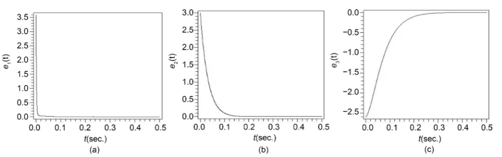
, d d d d d d1, 2, 3, 1′ ′ ′, 2, 3 are random from

−_{0.2 to 0.2. A time step of size 0.0001 (sec.) is employed and fourth-order Runge-} Kutta method is used to solve Equation (21) and Equation (22). Let k1=580,

2 30

k = , k3 =20, Figure 4 shows the history of e t1

( )

, e t2

( )

, e t3

( )

in the

error system (24) within 0.5 sec. From Figure 4, we can see that e t1

( )

, e t2

( )

,

( )

3

e t are steady near zero at last.

4. Conclusion

In this paper, a practical scheme is proposed for feedback synchronization with parameters perturbation and external disturbances. Lorenz system and the orig-inal Chua’s circuit are used for detailed description. The simulation results show the feasibility of the method. According to Ref. [15], if all the feedback coeffi-cients are larger than the largest Lyapunov exponent, two identical systems will be synchronized under ideal circumstance. In the paper, our scheme proved that high feedback coefficients will ensure more robust synchronization theoretically. The practical feedback should be bounded in a proper limit, so we have to con-trol the error within a proper bound to obtain suitable feedback. The feedback will be smaller when the error is smaller. It’s not hard for us to find a chance when the error between the drive system and the response system is small enough.

Acknowledgements

The work was supported by Natural Science Foundation of Liaoning Province (No. 201602034).

References

[1] Pecora, L.M. and Carroll, T.L. (1990) Synchronization of Chaotic Systems. Physical Review Letters, 64, 821-830. http://dx.doi.org/10.1103/PhysRevLett.64.821

[2] Carroll, T.L. and Pecora, L.M. (1991) Synchronizing Chaotic Circuits. IEEE Trans-actions on Circuits and Systems, 38, 453-456. http://dx.doi.org/10.1109/31.75404

[3] Wang, G.R., Yu, X.L. and Chen, S.G. (2001) Chaotic Control, Synchronization and Utilizing. National Defence Industry Press, Beijing.

[4] Wang, X.Y. (2003) Chaos in the Complex Nonlinearity System. Electronics Industry Press, Beijing.

[5] Chen, G.R. and Lü, J.H. (2003) Dynamical Analyses, Control and Synchronization of the Lorenz System Family. Science Press, Beijing.

(10)

and Synchronization. World Scientific, Singapore.

[7] Kapitaniak, T. (1996) Controlling Chaos: Theoretical and Practical Methods in Nonlinear Dynamics. Academic Press, London.

[8] Celka, P. (1996) Delay-Differential Equation versus 1D-Map: Application to Chaos Control. Physica D, 90, 235-241. http://dx.doi.org/10.1016/0167-2789(95)00243-X

[9] Agiza, H.N. and Yassen, M.T. (2000) Synchronization of Rössler and Chen Chaotic Dynamical Systems Using Active Control. Physics Letters A, 278, 191-197.

http://dx.doi.org/10.1016/S0375-9601(00)00777-5

[10] Khadra, A., Liu, X.Z., et al. (2005) Impulsive Control and Synchronization of Spati-otemporal Chaos. Chaos, Solitons & Fractals, 26, 615-636.

http://dx.doi.org/10.1016/j.chaos.2004.01.020

[11] Guo, W.L., Chen, S.H., et al. (2009) A Simple Adaptive-Feedback Controller for Chaos Synchronization. Chaos, Solitons & Fractals, 39, 316-321.

[12] Agrawal, S.K., Srivastava, M., et al. (2012) Synchronization of Fractional Order Chaotic Systems Using Active Control Method. Chaos, Solitons & Fractals, 45, 737- 752. http://dx.doi.org/10.1016/j.chaos.2012.02.004

[13] Norelys, A.C., Manuel, A., et al. (2016) Adaptive Synchronization of Fractional Lo-renz Systems Using a Reduced Number of Control Signals and Parameters. Chaos, Solitons & Fractals, 87, 1-11. http://dx.doi.org/10.1016/j.chaos.2016.02.038

[14] Kajbaf, A., Akhaee, M.A., et al. (2016) Fast Synchronization of Non-Identical Chao-tic Modulation-Based Secure Systems Using a Modified Sliding Mode Controller. Chaos, Solitons & Fractals, 84, 49-57. http://dx.doi.org/10.1016/j.chaos.2015.12.002

[15] Wang, F.Q. and Liu, C.X. (2006) A New Criterion for Chaos and Hyperchaos Syn-chronization Using Linear Feedback Control. Physics Letters A, 360, 274-278.

http://dx.doi.org/10.1016/j.physleta.2006.08.037

[16] Jiang, G.P. and Zheng, W.X. (2005) An LMI Criterion for Linear-State-Feedback Based Chaos Synchronization of a Class of Chaotic Systems. Chaos, Solitons & Frac- tals, 26, 437-443. http://dx.doi.org/10.1016/j.chaos.2005.01.012

[17] Zhang, H. and Ma, X.K. (2004) Synchronization of Uncertain Chaotic Systems with Parameters Perturbation via Active Control. Chaos, Solitons & Fractals, 21, 39-47.

[18] Lorenz, E.N. (1963) Deterministic Nonperodic Flow. Journal of the Atmospheric Sciences, 20, 130-141.

http://dx.doi.org/10.1175/1520-0469(1963)020<0130:DNF>2.0.CO;2

[19] Shil’nikov, L.P. (1994) Chua’s Circuit: Rigorous Results and Future Problems. In-ternational Journal of Bifurcation & Chaos, 4, 489-519.

(11)

Submit or recommend next manuscript to SCIRP and we will provide best service for you:

Accepting pre-submission inquiries through Email, Facebook, LinkedIn, Twitter, etc. A wide selection of journals (inclusive of 9 subjects, more than 200 journals)

Providing 24-hour high-quality service User-friendly online submission system Fair and swift peer-review system

Efficient typesetting and proofreading procedure

Display of the result of downloads and visits, as well as the number of cited articles Maximum dissemination of your research work