Estimation of the Optimum Rotational Parameter of the Fractional Fourier Transform Using its Relation to the Wigner Distribution

(1)

International Journal of Emerging Technology and Advanced Engineering

Website: www.ijetae.com (ISSN 2250-2459,ISO 9001:2008 Certified Journal, Volume 5, Issue 9, September 2015)

77

Estimation of the Optimum Rotational Parameter of the

Fractional Fourier Transform Using its Relation to the Wigner

Distribution

Seema Sud

1

1_{The Aerospace Corporation, 4851 Stonecroft Blvd. Chantilly, VA 20151}

Abstract—The Fractional Fourier Transform (FrFT) can provide significant interference suppression (IS) over the conventional Fast Fourier Transform (FFT) when the signal-of-interest (SOI) or interference is non-stationary. However, its limitation for practical use is estimating the optimum rotational parameter ‘a’. Current techniques choose ‘a’ that gives the minimum mean-square error (MMSE) between the desired SOI and its estimate. Such techniques are computational, and they do not provide good estimates when signal-to-noise ratio (SNR) or sample support is kept low, as is required in non-stationary environments. In this paper, we propose a novel method to estimate ‘a’ using a technique that chooses ‘a’ for which the projection of the product of the Wigner Distribution (WD) of the SOI and interference are minimum. This also corresponds to the value of ‘a’ for which the product of the energies of the SOI and interference in the FrFT domain is minimized. With the proposed algorithm, we can estimate ‘a’ with fewer samples and much better accuracy and speed than MMSE methods. Following estimation of ‘a’, we employ a reduced rank multistage Wiener filter (MWF), which is required to remove the non-stationary interference. Since the SOI and interference may be completely separable by filtering along the optimum FrFT axis, ‘ta’, we can obtain

significant IS regardless of signal-to-noise ratios (SNRs), where all other known techniques fail. We demonstrate the performance improvement of the proposed algorithm over MMSE methods by simulation, using several examples of non-stationary signals, and also compare the proposed algorithm to the FFT, which fails in non-stationary environments.

Keywords—Fractional Fourier Transform, Wigner Distribution, MMSE, MWF, FFT.

I. INTRODUCTION

The Fractional Fourier Transform (FrFT) has a wide range of applications in fields such as optics, quantum mechanics, image processing, and communications. It is a very useful method for separating a signal-of-interest (SOI) from interference and/or noise when the statistics of either are nonstationary [12].

The FrFT enables us to translate the received signal to an axis in the time-frequency plane where the SOI and interference may be separable [1], when they are not separable in the frequency domain, as produced by the conventional Fast Fourier transform (FFT), or in the time domain.

When applying the FrFT to perform interference suppression, we must first estimate the rotational parameter „a‟. Conventional methods rely on choosing the value of „a‟, 0 ≤ a ≤ 2, which produces the MMSE between a desired (training) signal and its estimate. Of course, when the environment is non-stationary, it is necessary to perform this estimation with very few samples, i.e. before the statistics of the received signal change. When this is not done, large estimation errors, which result in poor interference suppression, can occur. MMSE-based algorithms, however, are known to require a large number of samples in practice [13]; hence, their performance will be suboptimal in non-stationary environments.

(2)

International Journal of Emerging Technology and Advanced Engineering

78

Furthermore, because separation of an SOI and interference using the appropriate time-frequency axis may be almost perfectly achievable, whereby separation in the conventional time axis or frequency axis was not, we can achieve much better IS at very low SNR.

An outline of the paper is as follows: Section II describes the FrFT and its relation to the WD. Section III describes the adaptive filtering problem, now in the Fractional Fourier Transform (FrFT) domain. Section IV presents the MMSE-FrFT solution presented in [15] for obtaining „a‟ and filtering the interference. This solution is used because it does not rely on knowledge of the noise statistics like its predecessors. We also discuss the MMSE-FFT solution. Section V describes the proposed method for estimating the optimum value of „a‟ using the FrFT and its relation to the WD, which we denote as WD-FrFT. The proposed reduced rank method for filtering out the interference using the computed „a‟ is also discussed. Section VI has simulation results showing the improvement of the proposed method over MMSE-based methods. Finally, conclusions and remarks on future work are given in Section VII.

II. BACKGROUND: FRACTIONAL FOURIER TRANSFORM (FRFT)AND WIGNER DISTRIBUTION (WD)

The FrFT of a function f(x) of order „a‟ is defined as [12]

Where the kernel Ba(x,x′) is defined as

 = aπ/2, and . This applies to the range

0 < || < π, or 0 < |a| < 2. In discrete time, we can model the N × 1 FrFT of an N × 1 vector x as

Where Fa is an N × N matrix whose elements are given by

([3] and [12])

And where uk[m] and uk[n] are the eigenvectors of the matrix S defined by [3]

and

Numerous methods are presented in the literature for implementing the FrFT efficiently (see for example [2] and [3]).

The Wigner Distribution (WD) is a time-frequency representation of a signal, and may be viewed as a generalization of the Fourier Transform, which is solely the frequency representation. The WD of a signal x(t) can be written as

It is well-known that the projection of the WD of a signal x(t) onto an axis ta gives the energy of the signal in the FrFT domain „a‟, |Xa(t)|2 (see e.g. [8] or [9]). Letting α = aπ/2, this is written as

In discrete time, the WD of a signal x[n] can be written as [11]

Where l1 = max(0,n − (N − 1)) and l2 = min(n,N − 1). This particular implementation of the discrete WD is valid for non-periodic signals. Aliasing is avoided by oversampling the signal x[n] using a sampling rate of fs [samples per second] that is at least twice the Nyquist rate [11].

(3)

International Journal of Emerging Technology and Advanced Engineering

[image:3.612.64.280.237.404.2]

79

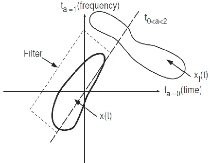
The WD shows how they both independently vary. Note that they both overlap in the time domain (ta=0) and in the frequency domain (ta=1), but there is some axis ta, 0 < a < 2, where they do not overlap. If we can find this optimum axis and rotate to it using the FrFT, we can filter out the interference in the new domain and achieve significant IS improvements over conventional time (e.g. MMSE) or frequency (e.g. FFT) filtering.

Fig. 1. Wigner Distribution of Signal x(t) and Interference xI(t) Shows

Optimum Axis ta Where Interference May Be Completely Filtered Out

III. PROBLEM FORMULATION

Without loss of generality, we consider a digital binary sequence whose elements are in (−1,+1) that we would like to estimate in the presence of non-stationary interference, and possibly a non-stationary channel. The signal is further corrupted by additive white Gaussian noise (AWGN). Here, we ignore the carrier, and hence model the SOI as a baseband binary phase shift keying (BPSK) signal. The number of bits per block is denoted N1, and if we oversample each bit by a factor of SPB (samples per bit), the number of samples per block in the BPSK signal is N = N1SPB, and the signal is denoted in discrete time, vector form as the N × 1 vector x(i). This SOI is corrupted by a non-stationary interferer xI(i), for which we will give several examples in Section VI, and by an AWGN signal n(i). In Section VI, we will model the case where the interference is not another signal but rather a nonstationary channel h(i) that is convolved with the SOI. Here, index i denotes the ith sample, where i = 1,2, …,N, and N is the total number of samples per block that we process. We then process M blocks (or trials) to obtain a statistical estimate of the MMSE. The received signal y(i) is then

We obtain an estimate of the transmitted signal x(i),

denoted (i), by first transforming the received signal to the FrFT domain, applying an adaptive filter, and taking the inverse FrFT. This is written as [15]

Where Fa and F−a are the N × N FrFT and inverse FrFT matrices of order „a‟, respectively, and

is an N × 1 set of optimum filter coefficients to be found. The notation diag(G) = (g0,g1,gN−1) means that matrix G has the scalar coefficients g0,g1,..., and gN−1 as its diagonal elements, with all other elements equal to zero.

IV. CONVENTIONAL METHODS FOR ESTIMATING „ ‟

A. MMSE-FrFT Method

MMSE-based methods aim to minimize the error

between the desired signal x(i) and its estimate (i). That is, we minimize the cost function

It is well known that the optimum set of filter coefficients g0 that minimizes the cost function in Eq. (13) can be obtained by setting the partial derivative of the cost function to zero [15]. That is, compute g0 such that

This is the MMSE-FrFT solution, given by [15]

Where

(4)

International Journal of Emerging Technology and Advanced Engineering

80

We thus choose the value of „a‟ as that which minimizes the cost function in Eq. (13). We point out that we must compute the cost function over the range of „a‟ from 0 < a < 2 by first computing g0,MMSE−FrFT from Eq. (15) to find the best value of „a‟. Note also that this solution requires a training sequence, x(i). We also mention that the LMS-FrFT solution presented in [10] will perform comparably to the MMSE-FrFT algorithm over time, hence we do not include it in our simulations.

B. MMSE-FFT Method

The MMSE-FFT solution is obtained simply by setting a = 1 in calculating g0 from Eqs. (15)−(18). This solution simply becomes one of applying the optimum filter given by Eq. (15) in the frequency domain, since F1 reduces to an FFT and F−1 is an inverse FFT (IFFT). In other words,

V. PROPOSEDMETHODFORESTIMATING „ ‟USING THE RELATION BETWEEN THE FRFT AND THE WD

The proposed technique seeks a way to estimate the optimum value of „a‟ by considering three factors: (1) we do not wish to use the received signal y(i) as this signal contains the SOI and interference together, making separation of the two harder; (2) we do not wish to require a large number of samples N, as this would result in errors in non-stationary channels, and more computational complexity in performing the estimate [13]; and (3) we do not wish to perform matrix inversions because even with a small number of samples N the computational complexity is O(N3) [13].

Note from Fig. 1 that the optimum rotational axis is that for which the desired signal and interference do not overlap, or in the practical case, overlap as little as possible. Hence, we could plot the Wigner Distribution of both the SOI and the interference (i.e. collect data with the SOI turned off) and search over the range of „a‟ to find the minimum. However, the discrete-time Wigner distribution evaluated at an arbitrary rotational axis is difficult to compute. Instead, from Eq. (8), note that we can more easily compute the WD along each axis ta by computing the energy of the FrFT along that axis. Hence, we propose to compute the energy of the FrFT of both the SOI and interference, compute their product, sum the values over the new time-frequency axis ta defined by the rotational parameter „a‟, and select as the optimum „a‟ the value for which the result is minimum. The proposed algorithm is summarized as follows:

Recall that Fa was defined in Eq. (4). If the distortion is not an interfering signal xI(i) but is instead a complex, time-varying channel h(i), written as an L × 1 channel vector

then the received signal is now written as

Where „*‟ denotes convolution. We can still apply the algorithm by computing

and replacing ℜXXI(a) in Step 4 above with

It is important to note that this algorithm requires a search over all „a‟ just like the MMSE method, but as we will show, it performs faster and provides significantly better estimates, resulting in better interference suppression. Note also that we need a training sequence here, just as in the conventional methods. In the absence of a training sequence, we may use the received signal, but we will suffer a performance loss. It is further important to note that Step (2) above requires calculation of the FrFT of the interference environment. Since the algorithm operates, as we will show, with very few samples, we can compute this in gaps where the SOI is off, as in a TDMA signal, or using empty sub-carriers, as in OFDM, etc.

(5)

International Journal of Emerging Technology and Advanced Engineering

81

The MWF was first introduced in [4] − [7] and it offers the advantages that it often exceeds MMSE performance without any computationally complex matrix inversion or eigen-decompositions, and we show here that these advantages exist in the FrFT domain as well. The efficient CSA implementation of the MWF was first presented in [14]. The recursion equations for the CSA-MWF are shown in Table I. Rank reduction is achieved because we can set D < N. We initialize the filter in the conventional way, except that we transform all the variables to the FrFT domain first. So, using the value of „a‟ obtained above, we let

and

The CSA-MWF computes the D scalar weights wj, j =

1, 2, ..., D, from which we form the optimum filter

TABLEI

RECURSION EQUATIONS FOR THE CSA-MWF

VI. SIMULATIONS

We present simulation examples to compare the proposed MMSE-FrFT and MMSE-FFT methods to the proposed WD-FrFT method for calculating the optimum FrFT rotational parameter „a‟.

We compute the adaptive filter coefficients for the three techniques from Eq.‟s (15), (19), and (26) respectively. We then use those coefficients to compute the resultant error between the true and estimated SOI from Eq.‟s (12) and (13). As already mentioned, we let the signal-of-interest (SOI) be a digital binary sequence whose elements are uniformly generated and in (−1,+1) that we would like to estimate in the presence of non-stationary interference and AWGN. Here, we ignore the carrier, and hence model the SOI as a baseband binary phase shift keying (BPSK) signal. We upsample the signal to generate N samples per block with N1 bits per block. Initially, we assume that N = 8 and N1 = 4 so that we oversample by 2 samples per bit (SPB). We vary the strength of the interfering signal by setting its amplitude based upon a desired carrier-to-interference ratio (CIR), and we set the amplitude of the AWGN based upon a desired Eb/N0. Specifically, we set the amplitude of the SOI to A = 1 by normalizing by and set the amplitude of the interferer to AI = 10−CIR/20, where the CIR is given in dB; note a negative CIR means that the interferer is stronger than the SOI. We further set the amplitude of the AWGN to be

Unless otherwise stated, we run the algorithm using M = 1000 trials, to obtain histograms of the error estimates using the three algorithms.

In the first example, we let the interfering signal take on the form of a chirp signal, given by

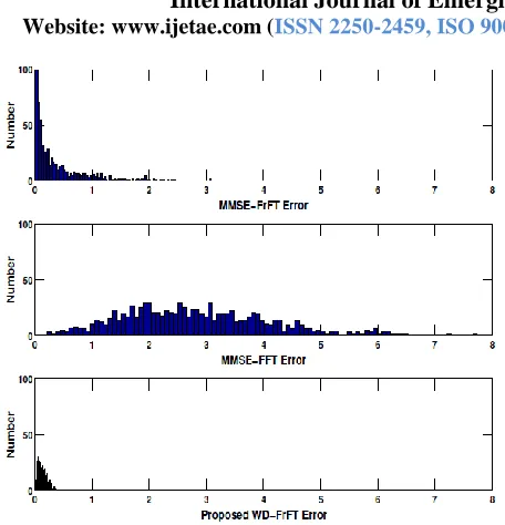
We set CIR = −10 dB, so the interference is much stronger than the SOI, and we let Eb/N0 = 10 dB. We sample at two samples per bit so that fs = 2Rb samples per second, where the bit rate is Rb = 1,000 bits per second. A plot comparing the histograms of the mean-square error of the three techniques is shown in Fig. 2. If we average over the 1000 trials, we obtain the error mean and variances as follows: µMMSE−FrFT = 0.278, µMMSE−FFT = 2.87, and µWD−FrFT=

0.13, σ2MMSE−FrFT = 0.20, σ2MMSE−FFT = 1.84, and σ2WD−FrFT

(6)

International Journal of Emerging Technology and Advanced Engineering

[image:6.612.54.282.111.348.2]

82

Fig. 2. MSE Comparison with Chirp Interferer, CIR = −10 dB, Eb/N0

= 10 dB)

The second example uses an interfering signal taking on the form of a Gaussian pulse, given by

Where β and  are the amplitude and phase of the pulse, respectively, uniformly distributed in (1,1.5). All other parameters are the same as in the previous example. We again scale the interference with amplitude AI to give CIR = −10 dB. A plot comparing the histograms of the mean-square error of the three techniques is shown in Fig. 3. Averaging over the 1000 trials gives µMMSE−FrFT = 0.096,

[image:6.612.323.557.130.355.2]

µMMSE−FFT = 1.60, and µWD−FrFT = 0.069,

σ

2MMSE−FrFT = 0.020, σ2MMSE−FFT = 1.22, and σ2WD−FrFT = 0.004.

Fig. 3. MSE Comparison with Gaussian Pulse Interferer, CIR =−10

dB, Eb/N0 =10 dB)

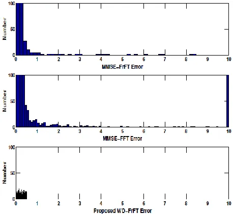
In the third example we assume there is no interference but instead there is a non-stationary channel h(i) that corrupts the signal. We model the channel as time-varying, bandpass signal whose center frequency is changing with time, given as an example in [8] as

(7)

International Journal of Emerging Technology and Advanced Engineering

[image:7.612.52.281.234.444.2]

83

Note that now, performance of the proposed WD-FrFT is much better than MMSE-FrFT and MMSE-FFT, which both fail due to their inability to remove a non-stationary channel that is corrupting the SOI in a non-additive way. Also, because the Eb/N0 is so low, all techniques suffer much larger errors. However, the WD-FrFT continues to produce much smaller estimation errors than the other two methods.

Fig. 4. MSE Comparison with Time-Varying Bandpass Channel,

Eb/N0 = −10 dB)

In the fourth example we assume there is interference and a non-stationary channel h(i) that corrupts the signal. The interference is the same as in the second example, and the channel is the same as in the previous example. We assume no knowledge of the channel, so that our algorithm uses solely the measured interference to compute the best „a‟. Furthermore, we let CIR = −10 dB and Eb/N0 = 10 dB. The result is shown in Fig. 5. We compute the following: µMMSE−FrFT = 0.059, µMMSE−FFT = 0.223, and µWD−FrFT =

0.053,

σ

2MMSE−FrFT = 0.006,

σ

2MMSE−FFT = 0.08, and

σ

2WD−FrFT = 0.003.

Now, because of the lack of knowledge of the corrupting channel, our technique degrades over the previous examples, but it still continues to outperform the other methods.

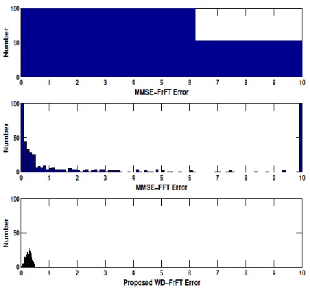
Finally, in the last example we assume the interference and channel are the same as in the previous example. We again assume no knowledge of the channel. But now, we let CIR = −10 dB and Eb/N0 = −10 dB. The result is shown in Fig. 6. Here, the FFT-MMSE method fails again, so we limit the error to a maximum of 10 to prevent large errors. Again, this means that the FFT results are worse than shown: µMMSE−FrFT = 7.27, µMMSE−FFT = 6.31, and µWD−FrFT =

[image:7.612.325.557.387.599.2]

0.276,

σ

2MMSE−FrFT = 1376,

σ

2MMSE−FFT = 20.7, and

σ

2WD−FrFT = 0.01. Here, we observe that both MMSE-FrFT and MMSE-FFT fail terribly because they cannot correct for the non-stationary interference and channel with such low SNR. The proposed technique degrades too, because of lack of channel knowledge and low SNR, but still performs far better than the other two techniques because it is able to estimate and remove the high powered interfering signal.

(8)

International Journal of Emerging Technology and Advanced Engineering

[image:8.612.55.281.133.345.2]

84

Fig. 6. MSE Comparison with Gaussian Pulse Interferer and

Time-Varying Bandpass Channel, CIR =−10 dB, Eb/N0 = −10 dB)

If we measure the computational complexity of each of these algorithms, which includes estimating „a‟ and then using the value computed to find the best estimate of the

transmitted signal, (i), we see that the proposed WD-FrFT algorithm performs 3 − 5 times faster than the MMSE-FrFT algorithm, whereas the MMSE-FFT algorithm is about 20 times faster than MMSE-FrFT. But, the MMSE-FFT algorithm operates on signals in the frequency domain only, and is thus sub-optimal in the presence of non-stationary interference or channels. The MMSE-FrFT algorithm also fails to perform well if the CIR or Eb/N0 is low. The proposed WD-FrFT algorithm, however, performs well over the range of parameters.

VII. CONCLUSION

In this paper, we present a simple, yet novel method for obtaining the best estimate of the rotational parameter „a‟ when computing a Fractional Fourier Transform to suppress non-stationary interference. The algorithm is robust in low sample support, low carrier-to-interference ratios (CIRs), and low Eb/N0. Because the algorithm finds an optimum time-frequency axis in which to filter a signal and eliminate interference, it greatly outperforms previous methods based solely on time or frequency analysis, because those methods are restricted to a single dimension and may not be able to adequately isolate the SOI from the interference.

The proposed method greatly outperforms existing time-frequency MMSE methods, which fail in low sample support or high interference because they rely on using the received signal, which does not isolate the SOI from the interference. MMSE methods also require large sample support, which is only available in stationary environments. Use of this technique could greatly enhance the ability to demodulate signals in high interference environments, and if a rotational axis can be found where the interference does not overlap the SOI, perfect interference cancellation may be done. Future work is to apply the newly developed algorithm to other applications in signal and image processing, and to real-life stressing signal processing problems.

Acknowledgments

The author thanks The Aerospace Corporation for funding this work and Alan Foonberg for reviewing the paper.

REFERENCES

[1] Almeida, L.B., “The Fractional Fourier Transform and Time-Frequency Representation”, IEEE Trans. on Signal Processing, Vol. 42, No. 11, Nov. 1994.

[2] Candan, C., Kutay, M.A., and Ozaktas, H.M., “The Discrete Fractional Fourier Transform”, Proc Int. Conf. on Acoustics, Speech, and Sig. Proc. (ICASSP), Phoenix, AZ, pp. 1713-1716, Mar. 15-19, 1999.

[3] Candan, C., Kutay, M.A., and Ozaktas, H.M., “The Discrete Fractional Fourier Transform”, IEEE Trans. on Sig. Proc., Vol. 48, pp. 1329-1337, May 2000.

[4] Goldstein, J.S., and Reed, I.S., “Multidimensional Wiener Filtering Using a Nested Chain of Orthogonal Scalar Wiener Filters”, University of Southern California, CSI-96-12-04, Dec. 1996. [5] Goldstein, J.S., and Reed, I.S., “A New Method of Wiener Filtering

and its Application to Interference Mitigation for Communications”, Proceedings of IEEE MILCOM, Vol. 3, pp. 1087-1091, Monterey, CA, Nov. 1997.

[6] Goldstein, J.S., Reed, I.S., and Scharf, L.L, “A New Method of Wiener Filtering”, Proceedings of the 1st AFOSR/DSTO Workshop on Defense Applications of Signal Processing, Victor Harbor, Australia, Jun. 1997.

[7] Goldstein, J.S., Optimal Reduced Rank Statistical Signal Processing, Detection, and Estimation Theory, Ph.D. Thesis, Dept. of Electrical Engineering, University of Southern California, Los Angeles, CA, Dec. 1997.

[8] Kutay, M.A., Ozaktas, H.M., Arikan, O., and Onural, L., “Optimal Filtering in Fractional Fourier Domains”, IEEE Trans. on Sig. Proc., Vol. 45, No. 5, May 1997.

(9)

International Journal of Emerging Technology and Advanced Engineering

85

[10] Lin, Q., Yanhong, Z., Ran, T., and Yue, W., “Adaptive Filtering in

Fractional Fourier Domain”, International Symposium on Microwave, Antenna, Propagation, and EMC Technologies for Wireless Communications Proc., pp. 1033-1036,

[11] O‟Toole, J.M., Mesbah, M., and Boashash, B., “Discrete Time and Frequency Wigner-Ville Distribution: Properties and Implementation”, Proc. Int. Symposium on Digital Sig. Proc. and Comm. Systems, Noosa Heads, Australia, Dec. 19-21, 2005. [12] Ozaktas, H.M., Zalevsky, Z., and Kutay, M.A., “The Fractional

Fourier Transform with Applications in Optics and Signal Processing”, John Wiley and Sons: West Sussex, England, 2001.

[13] Reed, I.S., Mallett, J.D., and Brennan, L.E., “Rapid Convergence Rate in Adaptive Arrays”, IEEE Trans. on Aerospace and Electronic Systems, Vol. 10, pgs. 853-863, Nov. 1974.

[14] Ricks, D.C., and Goldstein, J.S., “Efficient Architectures for Implementing Adaptive Algorithms”, Proc. of the 2000 Antenna Applications Symposium, pgs. 29-41, Allerton Park, Monticello, Illinois, Sep. 20-22, 2000.