Unsupervised Change Detection in Remote Sensing Images Using Pulse Coupled Neural Network

(1)

International Journal of Emerging Technology and Advanced Engineering

Website: www.ijetae.com (ISSN 2250-2459,ISO 9001:2008 Certified Journal, Volume 4, Issue 2, February 2014)

260

Unsupervised Change Detection in Remote Sensing Images

Using Pulse Coupled Neural Network

Geeta Desai

1

, Sonal Gahankari

2

1

Sr. Lecturer A.I.A.R.K.P polytechnic Navimumbai, India

2_{Assistant professor Saraswati College Of Engineering Navimumbai, India}

Abstract— In this paper we propose a context sensitive technique for unsupervised change detection in multitemporal satellite images of same scene using Pulse coupled neural network. PCNN is a novel artificial neural network which is developed in 1990 and based on visual cortex of cats. The binary images generated by each iteration of the PCNN algorithm create specific signatures of the scene which are compared for the generation of the change map .As a case study for the unsupervised change detection multitemporal images acquired by cartosat of Uttarkhand showing recent flooding area in Kedernath brought by heavy rainfall and multitemporal optical images acquired by Landsat on a part of Alaska are considered results are also shown on images acquired on sardina island and on Landsat images of Mexico.

Keywords—Pulse-coupled neural networks (PCNNs), unsupervised change detection, multitemporal images and remote sensing.

I. INTRODUCTION

Timely and accurate Change detection of earth features is very important for understanding interaction between human and natural phenomena. Detecting regions of change in images of same scene taken at different times is of widespread interest due to a large number of applications, like land use change analysis, study on shifting cultivation, monitoring of pollution, assessment of burned areas, monitoring of shifting cultivations, burned area identification, analysis of deforestation processes, assessment of vegetation changes, monitoring of urban growth and oceanography [3].The existing methods for change detection in remotely sensed data can be classified in supervised or in unsupervised manner in the literature several supervised and unsupervised techniques for detecting changes in remote sensing images have been proposed. The supervised methods require the availability of a ground truth for the setup of the system parameters whereas unsupervised approaches perform change-detection without using any additional ground information.

Compared to unsupervised methods supervised

approaches result in higher change detection accuracies are more robust to different atmospheric and light conditions at time of acquisition but still unsupervised techniques are more appealing as the ground truth information is not available in many change-detection applications. Most widely used unsupervised change-detection techniques are based on three-steps which are Pre-processing, image comparison and image analysis. In pre-processing step

operations like co-registration, noise reductions,

(2)

International Journal of Emerging Technology and Advanced Engineering

261

Processing tasks such as image segmentation, feature generation, image fusion, motion detection, pattern recognition face detection etc. [6]. In the comparison with other image processing algorithms, the PCNN algorithm is anti-noise and robust against the translation, scale, and rotation of the input patterns [10]. The visual cortex is that part of the brain that receives information from the eye and converts the eye image into a stream of pulses The pulses generated by each iteration of the PCNN algorithm create feature vector of the scene, which are compared for the generation of the change map. [1].

II. PCNN MODEL

A PCNN is a relatively new biological neural network based on understanding of the visual cortical models of cat .PCNN is derived from Eckhorn model in the 1990s it an single layer, two dimensional, laterally connected network of integrate and fire neurons .The size of the PCNN is the same size as the input image .Basic building block of an neural network is the neuron. Biological neuron is composed of dendrites, a cell body an axon and synaptic buttons. The cell body or soma acts as a threshold function a neuron receives signals from its neighbours via synapses and performs weighted algebraic summation on the inputs the architecture of the network is rather simpler than most other NN implementations. PCNNs do not have multiple layers, which pass information to each other. PCNNs only have one layer of neurons, which receive input directly from the original image, and form the resulting binary image. The PCNN neuron model is made up of feeding and linking receptive fields and pulse generator. The feeding Compartment receives both an external and local stimuli; whereas the linking compartment only receives the local stimulus which represents dendrites. The PCNN is mathematically modelled for the ith and, jth neuron by following equations.

Fig1 Representation of a PCNN neuron

The value of feeding compartment Fij is determined by the addition of the input image intensity at pixel (i,j),the weighted contributions of other neurons from the previous iteration and the feeding input of the prior iteration scaled by a decay constant as shown in equation 1.

Fij[n]= e-αF Fij[n-1]+ Sij + VF ∑MijYk[n-1] (1)

The value of linking compartment Lij is computed by addition of the weighted contribution of neighboring neurons from previous iteration and the linking input of the prior state scaled by decay coefficient as shown in equation 2

Lij[n]= e -αL

Lij[n-1] + VL ∑WijYk[n-1] (2)

Where Si,j is the input to the neuron (i, j) belonging , Each of these neurons communicates with neighboring neurons (kl) through the synaptic weights M and W, respectively. M and W are dependent on distance between neurons traditionally they follow very symmetric patterns. Y indicates the output of a neuron from a previous iteration [n − 1]. The distinction between the feeding and the linking is that the feeding connections have a slower characteristic response time constant than those of the linking inputs. The constant VF and VL are the normalizing constants If the receptive fields of M and W change then this constants are used to scale the resultant correlation to prevent saturation .U is the internal activity of neuron and determined by combining the states of feeding and linking compartments . The combination is controlled by the linking strength β. The internal activity is given by

Uij[n]= Fij[n]{1+βLij[n]} (3)

The pulse generator of neuron consists of a step function generator and a threshold signal generator the internal state of the neuron is compared to a dynamic threshold θ to produce the output Y

(4)

Ɵij= e-αƟ Ɵij[n-1] + VƟ Yij[n] (5)

In the pulse generator, if Uij is greater than the threshold, the output of neuron (i, j) turns into 1, neuron (i, j) fires, thenYij feedbacks to make him rise over Uij immediately, and them output of neuron (i,j) turns into 0. It will then take several iterations before the threshold values decay enough to allow the neuron to fire again. All compartments have a memory of the previous state, which decays in time by the

exponent term that decay is modeled by constant term αL ,

(3)

International Journal of Emerging Technology and Advanced Engineering

262

The PCNN algorithm is a iterative procedure in which output of one iteration stimulates the next iteration single iteration include computing (1)–(5) . From series of output images from PCNN, Johnson created an image signature also called the time signal It is important to observe that this time signal associated to the PCNN has the properties of invariance to changes in rotation, scale, shift, or skew of an object within the scene [7]. This quality makes the PCNN a powerful tool in change detection to reduce false alarms [1]

Fig2 PCNN Algorithm

III. PROPOSED CHANGE DETECTION ALGORITHM USING

PCNN

The application of PCNN to change detection is performed by measuring the similarity between PCNN signal associated to the former image and one associated to the latter. Equation 6 is used to convert pulsed image into single vector information

G[n]=∑Yij[n] (6) N

This can be effectively done by using correlation function operating between outputs of PCNN Equation 6 is used to convert pulsed image into single vector information A rather simple and effective way to do this is to use a correlation function operating between the outputs of the PCNN.

Fig3 Flowchart of proposed algorithm

IV. DESCRIPTION OF DATASET

(4)

International Journal of Emerging Technology and Advanced Engineering

263

4.1) Experimental data set of the Sardinia island, Italy. The first data set used in the experiments was made up of two multispectral images acquired by the Landsat Thematic Mapper (TM) sensor of the Landsat-5 satellite in September 1995 and July 1996. The test site is a section

(340 × 240 pixels) of a scene including Lake Mulargia on

the Island of Sardinia (Italy). Between the two aforementioned acquisition dates, the water level in the lake increased

4.2) Experimental data set of Mexico area.

The second data set used in our experiment is made up of two multispectral images acquired by the Landsat Enhanced Thematic Mapper Plus (ETM+) sensor of the Landsat - 7 satellite in an area of Mexico on 18th April 2000 and 20th May 2002.From the entire available Landsat scene, a section of 480×480 pixels has been selected as test site. Between the two aforementioned acquisition dates, fire destroyed a large portion of the vegetation in the considered region

4.3) Experimental data set of Alaska

The third datasetcontains a set of multispectral images collected on the part of Alaska to observe the land changes. Two images were acquired on 22 July 1985 and 13 July 2005 by Landsat 5 TM. A small area with 300 ×340 pixels are selected from images and presented in Figs. 6(a) and (b), respectively.. The ground truth of the change detection

mask which is shown in Fig. 6(d) was created by a manual

analysis of the input images based on Figs. 6(a) and (b). 4.4) Experimental data set of kedernath data set

The kedernath data set used in the experiments was made up of two mutitemporal images acquired by the cartosat sensor of the Cartosat-1 satellite in 2011 and June 2013 The test site is a section (520 × 620 pixels) of a scene including kedernath which is located in Himalayas about 3584m above sea level near head of river Mandakini . Between the two aforementioned acquisition dates Kederrnath town suffered heavy destruction during June 2013from flash floods caused by torrential rains in Uttarkhand state of India.

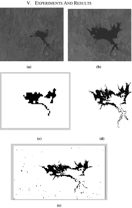
V. EXPERIMENTS AND RESULTS

(a) (b)

(c) (d)

(e)

Fig 4. (a) Band 4 of the Landsat TM image acquired in September 1995, (b) band 4 of the Landsat TM image acquired in July1996, (c) change detected image generated by using PCNN technique and (d) reference map (e) change detected image using image difference

method

[image:4.612.324.592.135.556.2]

(5)

International Journal of Emerging Technology and Advanced Engineering

264

(a) (b)

(c) (d)

(e)

Fig5 Images of Mexico. (a) Band 4 of the Landsat ETM+ image acquired in April 2000, (b) band 4 of the Landsat ETM+image acquired in May 2002, (c) reference image (d) change detected image generated by PCNN technique (e) change detected image using image

difference method

(a) (b)

(c) (d)

Fig6 Images of Alaska. (a) Landsat ETM+ image acquired in 22 July 1985 (b) Landsat ETM+image acquired in 13 July 2005, (c) reference image (d) change detected image generated by PCNN technique (e)

(6)

International Journal of Emerging Technology and Advanced Engineering

265

To assess the effectiveness of the proposed approach, we have made both visual and quantitative analysis of the experimental results. In visual analysis we have compared change detection map with the ground truth image . We then presented a quantitative analysis with respect to overall error. The change detection maps obtained for above mentioned data set by the proposed technique and image difference method are shown in Figs. 4 ,5, and 6 respectively. One can visually compare the change detection map generated by the proposed algorithms with the corresponding ground truth. This gives a rough idea about the quality of the generated change detection map.

[image:6.612.326.565.348.465.2]

Fig 7 Images of Kedernath. (a) Cartosat image acquired on 2011 (b) Cartosat image acquired on 2013, (c) reference image (d) change detected image generated by PCNN technique (e) change detected

image using image difference method

VI. QUANTITATIVE ANALYSIS

In order to evaluate the performances of the proposed change detection algorithm, we have chosen the following parameters.

1) Correct Detection Rate [%]:

CDR=True positives/(True positives +False positives)

2) Correct rejection rate

CRR=True negatives/(True positives +False positives)

3) False positive rate

FPR = false positives/(True negatives +False positives)

4) Miss rate

MR= false positives/(True positivess +False positives)

Approximation of Total Success Rate [%]: TSR = (CDR + CRR)/2,

where:

TP = true positives = changes correctly detected TN = true negatives = no-changes detected correctly FP = false positives = no-changes detected as changes FN = false negatives=changes detected as non-changes

Table1

Data set

CDR CRR FPR MR TSR

Sardina 98.37 73.84 26.1502 1.62 87

Mexico 98.96 71.74 28.25 1.03 85.35

Alaska 99.70 78.32 21.671 0.2955 89.0168

VII. CONCLUSION

(7)

International Journal of Emerging Technology and Advanced Engineering

266

However, the preliminary results indicate that applying the same parameter values to different VHR images keeps the performance still satisfactory. Fluctuations in results seem to be more critical for VƟ and αƟ, compared to other parameters

REFERENCES

[1] Fabio Pacific, Fabio Del Frate ―Automatic change detection in very high resolution images with pulse coupled neural networks‖ IEEE Tran. Geoscience and remote sensing vol.7 pp. 58-62.

[2] Susmitha Ghosh, Lorenzo Bruzzone ―A context sensitive technique for unsupervised change detection based on Hopfield type neural networks‖ IEEE Tran. Geoscience and remote sensing vol.45 pp. 778-789

[3] Swarnajyothi patra ,sushmita Ghosh, Ashish Ghosh ―Unsupervised change detection in remote sensing images using one dimensional self-organizing feature map neural network ―conference on computing IEEE computer society

[4] Swarnajyothi patra ,sushmita Ghosh, Ashish Ghosh ―An Unsupervised change detection in remote sensing images using modified self-organizing feature map neural network‖ conference International journal of approximation reasoning 2009 pp. 37-50

[5] Victor mihal ― A neural network approach for land cover change detection in multitemporal multispectral remote sensing imagery‖recent advances in signal processing ,computional geometry and system theory

[6] Turgay Celik ― Image change detection using Gaussian mixture model and genetic algorithm‖ Elsevier J. Vis. Commun. Image R. 21 (2010) 965–974

[7] Book by T. Lindbad and J.M. kinser ―image processing using pulse coupled neural networks‖ springer second edition.

[8] Trong -Thuc Hoang, Ngoc-Hung Nguyen, Xuan-Thuan Nguyen and Trong Tu] ―A Real-time Image Feature Extraction Using PCNN‖ International journal of emerging trends and technology in computer science PP

[9] Lorenzo Bruzzone, Member, IEEE, and Diego Fernàndez Prieto, Student Member, IEEE, ‖ Automatic Analysis of the Difference Image for Unsupervised Change Detection‖ IEEE transactions on geoscience and remote sensing, vol. 38, NO. 3,