Waveform lidar over vegetation : An evaluation of inversion methods for estimating return energy

(1)

Wav efo r m lid a r ov e r v e g e t a ti o n :

An e v al u a ti o n of i nv e r si o n

m e t h o d s fo r e s ti m a ti n g r e t u r n

e n e r g y

H a n c o c k, S, Ar m s t o n , J, Li, Z, G a ul t o n , R, L e wi s, P, Di s n ey, M ,

D a n s o n , F M , S t r a h l er, A, S c h a af, C, An d e r s o n , K a n d G a s t o n , KJ

h t t p :// dx. d oi.o r g / 1 0 . 1 0 1 6 /j. r s e . 2 0 1 5 . 0 4 . 0 1 3

T i t l e

Wav ef o r m lid a r ov e r v e g e t a ti o n : An e v al u a tio n of

inv e r si o n m e t h o d s fo r e s ti m a ti n g r e t u r n e n e r g y

A u t h o r s

H a n c o c k , S, Ar m s t o n , J, Li, Z, G a ul t o n , R, L e wi s, P, Dis n ey,

M , D a n s o n , F M , S t r a h l er, A, S c h a af, C, An d e r s o n , K a n d

G a s t o n , KJ

Typ e

Ar ticl e

U RL

T hi s v e r si o n is a v ail a bl e a t :

h t t p :// u sir. s alfo r d . a c . u k /i d/ e p ri n t/ 3 4 9 7 2 /

P u b l i s h e d D a t e

2 0 1 5

U S IR is a d i gi t al c oll e c ti o n of t h e r e s e a r c h o u t p u t of t h e U n iv e r si ty of S alfo r d .

W h e r e c o p y ri g h t p e r m i t s , f ull t e x t m a t e r i al h el d i n t h e r e p o si t o r y is m a d e

f r e ely a v ail a bl e o nli n e a n d c a n b e r e a d , d o w nl o a d e d a n d c o pi e d fo r n o

n-c o m m e r n-ci al p r iv a t e s t u d y o r r e s e a r n-c h p u r p o s e s . Pl e a s e n-c h e n-c k t h e m a n u s n-c ri p t

fo r a n y f u r t h e r c o p y ri g h t r e s t r i c ti o n s .

(2)

Waveform lidar over vegetation: An evaluation of inversion methods for

estimating return energy

Steven Hancock

a,

⁎

, John Armston

b

, Zhan Li

c

, Rachel Gaulton

d

, Philip Lewis

e

, Mathias Disney

e

,

F. Mark Danson

f

, Alan Strahler

c

, Crystal Schaaf

g

, Karen Anderson

a

, Kevin J. Gaston

a

Environment and Sustainability Institute, University of Exeter, United Kingdom b

Remote Sensing Centre, Science Delivery, Department of Science, Information Technology and Innovation, 41 Boggo Road, QLD 4102, Australia and Joint Remote Sensing Research Program, School of Geography, Planning and Environmental Management, University of Queensland, St Lucia, QLD 4072, Australia

c

Department of Earth and Environment, Boston University, United States d_{School of Civil Engineering and Geosciences, Newcastle University, United Kingdom} e

UCL Geography and NERC National Centre for Earth Observation, United Kingdom f

Ecosystems and Environment Research Centre, School of Environment & Life Sciences, University of Salford, United Kingdom g

School for the Environment, University of Massachusetts Boston, United States

a b s t r a c t

a r t i c l e i n f o

Article history:

Received 8 December 2014 Received in revised form 9 April 2015 Accepted 10 April 2015

Available online xxxx

Keywords: Lidar Full waveform Forests Reﬂectance Signal processing

Full waveform lidar has a unique capability to characterise vegetation in more detail than any other practical method. The reflectance, calculated from the energy of lidar returns, is a key parameter for a wide range of appli-cations and so it is vital to extract it accurately. Fifteen separate methods have been proposed to extract return energy (the amount of light backscattered from a target), ranging from simple to mathematically complex, but the relative accuracies have not yet been assessed. This paper uses a simulator to compare all methods over a wide range of targets and lidar system parameters. For hard targets the simplest methods (windowed sum, peak and quadratic) gave the most consistent estimates. They did not have high accuracies, but low standard viations show that they could be calibrated to give accurate energy. This may be why some commercial lidar de-velopers use them, where the primary interest is in surveying solid objects. However, simulations showed that these methods are not appropriate over vegetation. The widely used Gaussianfitting performed well over hard targets (0.24% root mean square error, RMSE), as did the sum and spline methods (0.30% RMSE). Over vegetation, for large footprint (15 m) systems, Gaussianfitting performed the best (12.2% RMSE) followed closely by the sum and spline (both 12.7% RMSE). For smaller footprints (33 cm and 1 cm) over vegetation, the relative accuracies were reversed (0.56% RMSE for the sum and spline and 1.37% for Gaussianfitting). Gaussianfitting required heavy smoothing (convolution with an 8 m Gaussian) whereas none was needed for the sum and spline. These simpler methods were also more robust to noise and far less computationally expensive than Gaussian fitting. Therefore it was concluded that the sum and spline were the most accurate for extracting return energy from waveform lidar over vegetation, except for large footprint (15 m), where Gaussianfitting was slightly more accurate. These results suggest that small footprint (≪15 m) lidar systems that use Gaussianfitting or proprie-tary algorithms may report inaccurate energies, and thus reflectances, over vegetation. In addition the effect of system pulse length, sampling interval and noise on accuracy for different targets was assessed, which has impli-cations for sensor design.

1. Introduction

Lidar has been shown to be a valuable tool for characterising vege-tation, offering many advantages over other techniques due to its non-destructive measurement of structural and spectral information (Dubayah & Drake, 2005). Maps of global forest height have been

determined from the spaceborne ICESat (Harding & Carabajal, 2005; Los et al., 2012), forest cover can be accurately derived from airborne lidar without the need for site-speciﬁc calibration (Armston et al., 2013), airborne lidar's structural information improves land cover classiﬁcation accuracy (Mallet, Bretar, Roux, Soergel, & Heipke, 2011), airborne and terrestrial laser scanners (TLS) have also been used to characterise vegetation canopies and their effect on hydrological pro-cesses (Musselman, Margulis, & Molotch, 2013; Reid et al., 2014) and TLS can accurately measure woody volume (Raumonen et al., 2013), po-tentially allowing rapid biomass measurement. All of these studies rely on accurately extracting target properties from lidar signals.

⁎ Corresponding author.

E-mail addresses:[email protected](S. Hancock),[email protected]

(R. Gaulton),[email protected](F. Mark Danson).

http://dx.doi.org/10.1016/j.rse.2015.04.013

Contents lists available atScienceDirect

Remote Sensing of Environment

(3)

Lidar directly measures the 3D distribution of energy reﬂected from a target surface. The vast majority of research has focused on determin-ing the range to a sdetermin-ingle feature (Stilla & Jutzi, 2008; Wagner, Ullrich, Melzer, Briese, & Kraus, 2004), with very few studies assessing the accu-racy of the estimated return energy (backscattered radiation from the target). Recent research has tried to identify targets through clutter, such as the ground surface under vegetation (Jalobeanu & Gonçalves, 2014; Los et al., 2012), but they still assumed that there was a hard fea-ture that lay at a single range. Commercial lidar systems have been optimised to measure the range to hard features.

The return energy contains useful information about complex targets, such as vegetation. The amount of energy returned can be used to calculate the size of illuminated objects (Hancock et al., 2014; Ramirez, Armitage, & Danson, 2013) and determine canopy cover (Armston et al., 2013). The return energy of certain wavelengths is re-lated to leaf biochemistry and can be used to calculate leaf moisture (Gaulton, Danson, Ramirez, & Gunawan, 2013) and chlorophyll content (Nevalainen et al., 2014). It has been shown that lidar return energy is the most important lidar metric when classifying land cover type (Mallet et al., 2011; Neuenschwander, Magruder, & Tyler, 2009). There-fore an accurate method for retrieving return energy from lidar is vital for making physically based measurements of vegetation. In addition, vegetation canopies contain many small elements, making it likely that a lidar beam will hit multiple targets within a single return feature, potentially violating the assumptions of methods developed for single targets.

Many previous papers have assessed the accuracy of the range esti-mate from lidar data (Stilla & Jutzi, 2008; Wagner et al., 2004). Fewer have explored the accuracy of return energy and these previous energy extraction studies are described inSection 3.4. This study deals exclu-sively with methods for determining the energy of a return, with a view to improving the accuracy of physically based measurement methods of vegetation (which require no site specific calibration). This study assessed the methods in terms of their return energy accuracy, ro-bustness and computational expense for both single, hard returns and for complex, vegetation returns. Return energy accuracy was assessed in terms of absolute accuracy and also in terms of consistency, as the value retrieved by a method can be calibrated to give true energy as long as there is a consistent, well defined relationship between the re-trieved value and energy. Computational efficiency is an important con-sideration asJalobeanu and Gonçalves (2014)state that“the best performing methods are too computationally intensive to be used on large datasets”.

Empirical methods have been proposed to characterise vegeta-tion without the need for target biophysical parameters to be directly derived from the lidar signal, e.g. Height Of Median Energy, HOME (Drake et al., 2002) and the leading edge extent (Lefsky, Keller, Yong, de Camargo, & Hunter, 2007). However these empirical methods

require local calibration. Physically based methods, directly extracting target properties from the lidar signal, require no external calibration and so can be applied globally. The resulting parameters have a physical meaning that can be directly measured on the ground such as canopy cover, tree height or leaf area.

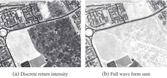
Fig. 1 shows maps generated using two different methods for determining return strength from a Leica ALS50-II airborne lidar.

Fig. 1(a) shows the intensity reported by Leica's proprietary dis-crete return algorithm (sum of multiple returns per beam) whilst

Fig. 1(b) shows the sum of full waveform intensity. For both, the return strength was calculated per beam and averaged into a 2 m raster. These lead to very different outputs, with forests providing a stronger return inFig. 1(b) than (a) and so researchers might draw different conclu-sions about the biophysical nature of the vegetation depending on which method they used. This paper will explore the different methods to measure lidar return energy and which are more accurate over dif-ferent surfaces. Several new lidar systems optimised for vegetation are in development covering terrestrial, airborne and satellite based sys-tems (Danson et al., 2014; Douglas et al., 2015; Murooka et al., 2013; Wallace, Nichol, & Woodhouse, 2012) and so this type of data will be-come ever more common.

2. Lidar systems

There are two broad classes of lidar, time offlight (TOF) and phase shift systems. Phase shift systems have been shown to struggle at deter-mining if and where a hit occurs in diffuse targets, such as vegetation due to their assumption that all reflected light comes from a single sur-face (Newnham, Goodwin, Armston, Muir, & Culvenor, 2012), and so these systems will not be covered here. TOF lidar systems emit a short pulse of light and measure the reflected energy, allowing the range to, and apparent reflectance of, the target surface to be determined. Within TOF lidars there are two further categories, discrete return and full waveform systems. Discrete return systems use proprietary algorithms to extract the range and energy of one or more targets along the laser beam's path (Disney et al., 2010; Jalobeanu & Gonçalves, 2012). Full waveform systems record all the reflected energy as a function of range, giving a more complete description of the scattering event (Harding, Blair, Garvin, & Lawrence, 1994) and allowing more accurate measurement of target properties over diffuse targets such as vegeta-tion (Hancock, Disney, Muller, Lewis, & Foster, 2011). The data and pro-cessing requirements are much greater for full waveform than for discrete return lidar, although some doubts have been raised about the accuracy of range and energy derived from the proprietary discrete return algorithms over vegetation (Disney et al., 2010). This study fo-cuses on methods for full waveform lidar, where the energy can be ex-tracted from waveform lidar in a number of ways, ensuring that the optimal information is available for the task.

[image:3.595.133.473.569.728.2]

(a)

Discrete return intensity

(b)

Full wave form sum

(4)

For full waveform systems, a digitiser records the intensity mea-sured by a photodetector as a digital number (DN) at a preset sampling interval, referred to as a“bin”. The outgoing laser pulse will have some distribution function whilst the detector will have a response function (typically assumed to be Gaussian). The convolution of these two com-ponents gives the system pulse (referred to as“the pulse”for the rest of this paper). The measured waveform is the convolution of this system pulse with the target proﬁle, sampled at the sampling interval, plus noise. These three effects are explained in the following sections.

2.1. System pulse

[image:4.595.124.464.53.198.2]

Fig. 2illustrates two Gaussian returns sampled at 1 ns (see online version for colourfigures). This shows the interaction between pulse length and sampling interval to define the amount of information avail-able (number of green crosses). The fewer samples there are across a feature the more uncertain the location and reflectance of that feature (Landi, 2002). Note that the amount of information available to the ex-traction algorithm depends on the ratio of the pulse length to the sam-pling interval, so that a 2 m pulse sampled every 1 ns contains the same amount of information as a 1 m pulse sampled every 0.5 ns and the two should be retrieved with identical accuracies, though the shorter pulse will be able to separate more closely spaced objects.

Table 1shows the characteristics of the majority of waveform lidar systems that have been used for vegetation. Note that pulse widths are reported in terms ofσ, deﬁned as half the distance between the points at which the power drops below 61% of the maximum rather than the full-width-half-maximum (FWHM).Fig. 3shows some exam-ples of lidar system pulses.Fig. 3(a) shows the very short (σ= 0.1 m)

Gaussian pulse of SALCA (Danson et al., 2014).Fig. 3(b) shows the longer (σ = 0.53 m), asymmetric pulse of the Leica ALS50-II.

Fig. 3(c) shows the short (σ= 0.23 m) but well sampled DWEL pulse (Douglas et al., 2015). This is near-Gaussian, but the detectorﬁlters out high-frequency returns, leading to an oscillation at the trailing edge.Fig. 3(d) shows the short (σ= 0.35 m) asymmetric pulse for a Riegl VZ-400. Of note is the Riegl VZ-400's long trailing edge, due to strong returns causing non-linearity in the detector electronics.

There have been recent developments to use single photon counting systems to measure the lidar waveform instead of traditional pho-todiode detectors. These are much more sensitive to low intensity sig-nals, requiring lower powered lasers and so making the instrument lighter and cheaper. NASA's SIMPL (Dabney et al., 2010) and ICESat II (Harding et al., 2011) instruments currently in development are exam-ples andMoussavi, Abdalati, Scambos, and Neuenschwander (2014)

demonstrated that they can measure forest height. However they re-quire repeated measurements to measure energy, either from aﬁxed position (Hernandez-Marin, Wallace, & Gibson, 2007; Wallace et al., 2012) or by averaging over an area (Moussavi et al., 2014), which intro-duces statistical errors on top of the error from inversion methods. Due to the different sampling methods described above these will not be in-vestigated here.

2.2. Target proﬁle

The target profile is the product of reflectance, phase function and projected area along the path of the laser beam (Jupp et al., 2009) and the amount of energy returned is the integral of the target profile. This is the true waveform, without any effects from the lidar system or

0 10 20 30 40 50 60 70 80 90 100

8.5 9 9.5 10 10.5 11 11.5 8.5 9 9.5 10 10.5 11 11.5

DN

Range (m)

0 20 40 60 80 100

DN

Range (m)

(a)

_σ

= 0.5m

(b)

σ

= 0.1m

[image:4.595.36.553.575.744.2]

Fig. 2.Two different pulse lengths,σ, sampled at 1 ns intervals.

Table 1

Full waveform lidar system characteristics. Pulse widths are in terms ofσ. Footprint sizes are for typicalﬂying altitudes for space and airborne systems and at 10 m for terrestrial systems.

Instrument Pulse width Footprint Digitiser Wavelength Reference

Spaceborne

ICESat 0.76 m 52 m–90 m 1 ns 1064 nm Harding and Carabajal (2005)

MOLI TBD 25 m TBD 1064 nm Murooka et al. (2013)

GEDI TBD 25 m TBD 1064 nm Krainak et al. (2012)

Airborne

Lidar 1.8 m 75 cm 2.5 ns 337 nm Nelson, Krabill, and Maclean (1984)

SLICER 1.27 m 10 m 0.7 ns 1064 nm Harding et al. (1994)

LVIS 1.27 m 10–30 m 2 ns 1064 nm Hofton et al. (2000)

Optech ALTM 3100 1.02 m 30–80 cm 1 ns 1064 nm Wagner et al. (2006)

Riegl LMS-Q560 0.51 m 50 cm 1 ns 1545 nm Wagner et al. (2006)

Leica ALS50-II 0.53 m 33 cm 1 ns 1064 nm Hill and Broughton (2009)

Terrestrial

Echidna 1.90 m ≈50 mm 0.5 ns 1064 nm Jupp et al. (2009)

Riegl VZ-400 0.35 m ≈2 mm 1 ns 1545 nm Calders et al. (2014)

SALCA 0.10 m ≈5 mm 1 ns 1064 nm & 1545 nm Danson et al. (2014)

(5)

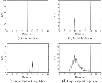
multiple scattering, from which target properties can be directly de-rived.Fig. 4(a) shows a single surface thatﬁlls theﬁeld of view and at a shallow enough angle of incidence that the difference in range across the laser footprint is less than a range bin, such as bare Earth, a rock face, building or tree trunk (a single Dirac-delta function). In this case the

peak intensity and energy are the same and this is what most commer-cial lidars have been designed to measure.Fig. 4(b) shows multiple short returns, such as a small footprint laser beam passing through branches or clipping the corner of a building. Vegetation canopies have many small elements that can lead to diffuse target proﬁles, such

Riegl VZ-400

Fig. 3.System pulse examples.

0 20 40 60 80 100

0 5 10 15 20 25 30 35 40 0 5 10 15 20 25 30 35 40

DN

Range (m)

(a)

Hard surface

0 2 4 6 8 10 12 14 16

DN

Range (m)

0 5 10 15 20 25 30 35 40 0 5 10 15 20 25 30 35 40

Range (m) Range (m)

(b)

Multiple objects

0 2 4 6 8 10 12 14 16 18

DN

(c)

Small footprint, vegetation

0 10 20 30 40 50 60 70 80

DN

(d)

Large footprint, vegetation

[image:5.595.125.476.443.727.2]

(6)

asFig. 4(c) and (d), where the peak intensity and energy are not directly related.Fig. 4(c) shows a typical small footprint (33 cm diameter circle) airborne return from vegetation, with a number of overlapping ele-ments giving a complex return.Fig. 4(d) shows a typical large footprint (10 m) return from vegetation, with a continuous smear of reﬂected energy.

In these cases the proﬁle cannot be described by a single range and so the assessment of range accuracy is not trivial. Therefore this paper will deal exclusively with the extraction of energy. It is possible to use separate algorithms for determining range and energy and so the results of this study are still general.Section 5.2will explore which of the cases inFig. 4occur for the different footprint sizes outlined inTable 1and how that affects energy retrieval accuracy.

2.3. Noise

All lidar systems suffer from noise (Baltsavias, 1999), consisting of background, detector and photon noise (Hancock, 2010), Section 4.1.3.

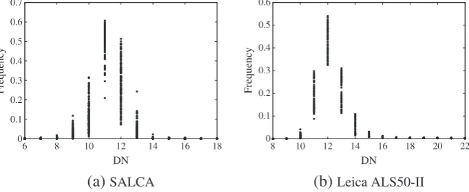
Fig. 5(a) shows the frequency distribution of all returns measured by SALCA in 37 separate scans between October 2010 and January 2014 andFig. 5(b) shows all data collected during four differentﬂights with the NERC ARSF Leica ALS50-II between July and October 2012. Leica waveforms were 37 m long and SALCA 15 m to 105 m long, sampled every 15 cm, giving 100–700 samples per waveform with energy from targets in only a few metres of bins and so the vast majority of bins contain only background and detector noise, dominating the distribu-tions. These scans were collected in a range of environments (indoors, outdoors, in cloud and bright sunshine for SALCA and over different sur-faces for the Leica ALS50-II). That all waveforms, with different ambient light levels, show a similar noise level suggests that this is not due to background light but must be due to detector noise. The implications for signal processing are discussed inSection 3.3.

3. Extraction methods

Table 2lists the different methods used for extracting energy (and so re_ﬂectance) and a three letter acronym by which they will be referred to in this paper. This list is comprehensive as far as the authors are aware. There are other methods that only measure range, but only methods ca-pable of estimating energy were tested here. The methods can be split into two main approaches, linear and iterative.

3.1. Linear methods

These are computationally efﬁcient, requiring only a single pass through the data. They also tend to be numerically stable with the majority giving an output no matter what the input, although some of the more complex methods rely on matrix inversion and so can fail for

certain inputs. Complete descriptions of all methods are given in

Appendix A.

After the processing for this paper had been completedJalobeanu and Gonçalves (2014)introduced a more robust version of the three point Gaussian using a very constrained Gaussianfitting to smooth and suppress ringing and Bayesian methods to constrain the three pointfit. This increased the robustness and computational efficiency of the method over single, hard targets but the effect on return energy ac-curacy was not discussed and it is not clear that there would be any im-provement. Because of this, this method was not tested here.

3.2. Iterative methods

These are more mathematically complex and computationally expensive than the linear methods (Neuenschwander et al., 2009). All studies so far have used the Levenberg–Marquardt iterative, non-linear optimisation tofit assumed pulse shapes to the waveform. The MINPACK implementation of the Levenberg–Marquardt algorithm, with constraint, was used for the investigation (Garbow, Hillstrom, More, Markwardt, & Moshier, 1980). For overlapping returns (from dif-fuse targets) points of inflection were used to identify the number of functions within a feature and multiple shapes werefitted (Hofton, Minster, & Blair, 2000). Turning points were used to set initial estimates. Complete descriptions of all methods are given inAppendix B.

3.3. Denoising

Background noise must be removed before identifying returns.Fig. 5

suggests that, for SALCA and the Leica ALS50-II, the background noise is very stable and so can easily be removed by thresholding. Thresholding will remove some true signal and so the noise tracking method present-ed in (Hancock et al., 2011) was used to set the threshold (mean detec-tor noise plusﬁve standard deviations) and then tracking back to the mean noise level to get the start and end of the feature. This reliably removes the effect of background noise for instruments with such stable behaviour, though less stable instruments may need more complex methods in order to prevent mistaking noise for a real return.

In addition, there will be distortions in the received signal due to de-tector and photon noise (Hancock, 2010, Section 4.1.3). Smoothing can help make inversions more robust but has the disadvantage of blurring the signal, reducing the ability to separate nearby objects. It should also be noted that smoothing does not add to the information content avail-able for the inversion and some suggest that it is better to use the raw data (Press, Tuekolsky, Vetterling, & Flannery, 1994).

3.4. Previous comparisons

A small number of previous studies have assessed the accuracy of energy extraction algorithms. However, the vast majority have focused

0 0.1 0.2 0.3 0.4 0.5 0.6 0.7

6 8 10 12 14 16 18

Frequency

DN DN

(a)

SALCA

0 0.1 0.2 0.3 0.4 0.5 0.6

8 10 12 14 16 18 20 22

Frequency

[image:6.595.124.465.588.728.2]

(b)

Leica ALS50-II

(7)

on more mathematically complex methods (Chauve et al., 2007; Roncat, Bergauer, & Pfeifer, 2011; Wagner, Ullrich, Ducic, Melzer, & Studnicka, 2006; Wu, van Aardt, & Asner, 2011). Only a handful of papers have in-vestigated the simple methods and none have comprehensively com-pared their performance to the mathematically complex methods.

Jutzi and Stilla (2005)compared the peak, rectangular sum and Gaussian (PEA, SUR and GAU) and concluded that, for their simple targets, the Gaussian performed slightly better than the peak and both performed better than the sum, though their focus was on range accura-cy.Lin, Shih, and Teo (2010)explored the three methods used in Riegl's RiANALZE software (PEA, SUR and GAU), however no validation was attempted and so they could not conclude which method was more ac-curate.Armston et al. (2013)looked at the difference between Gaussian

ﬁtting and the sum for calculating return energy in the estimation of canopy cover, concluding that the latter gave more accurate energies for vegetation but that the Gaussian gave as good a result in the majority of cases and so, as one of their datasets (Riegl LMS-Q680i) only reported Gaussian parameters, the Gaussians were used to calculate canopy cover.Jalobeanu and Gonçalves (2014)used the three-point Gaussian but did not compare to other methods.

As far as the authors are aware no other studies have tested the suit-ability of the simple methods to extract return energy from waveform lidar. This study expands on previous work by including all waveform lidar algorithms capable of calculating energy and using realistic simu-lations to compare their performance across a range of lidar systems, targets and noise levels in order to see how accurately each method can extract return energy for different situations, paying particular at-tention to whether a computationally efﬁcient method can achieve the same results as the more widely used, computationally expensive and mathematically complex methods.

4. Experiments

The performance of theﬁfteen algorithms (listed inTable 2) over a wide range of conditions was tested on both single and multiple, com-plex returns over the full range of pulse widths, pulse shapes, ampli-tudes and noise levels observed in current instruments. Simulators were used, for which the truth is known precisely, allowing accurate assessment of errors. In all cases the methods were tested on the raw waveforms and after smoothing by Gaussians with a range of widths.

The accuracy was assessed in terms of the bias (difference between true and retrieved energy), root mean square error (RMSE), failure rate (fraction of inversions that failed due to instability or gave a return energy greater than 1000, a nonsensical value that would skew the sta-tistics) and the mean standard deviation of the energy estimates for each true energy. The last of these indicates whether a method gave a consistent estimate of energy for a given return shape at different ranges and in the presence of noise. If a method has a low standard de-viation, bias can be removed by calibration, though it is preferable to

have a low RMSE. Note that due to the order of averaging, the standard deviation and RMSE were not directly comparable.

Throughout the paper a sampling interval of 1 ns was used. As noted inSection 2.1, this can represent any sampling interval after scaling the pulse lengths quoted by the ratio of the sampling intervals. Obviously the higher the sampling rate the more information there is available to a shorter pulse and so the smaller the minimum separation at which objects can be identiﬁed (Danson et al., 2014).

4.1. Single returns

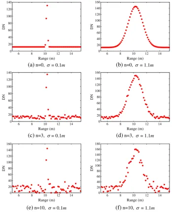
A simulator, written in C, was used to create example waveforms for single returns, as shown inFig. 3. Two different pulse shapes were used: (i) Gaussian (such as SALCA and ICESat); and (ii), the system pulse of the Leica ASL50-II to represent an asymmetric pulse (Fig. 3(b)). These will be refereed to as“Gaussian”and“asymmetric”pulses for the rest of this paper. Within the simulator the pulses could be centred at any point to test the method's ability to deal with sub-bin shifts, with any amplitude (measured in digital numbers, DN) and with any pulse width (σ). As the returns are from a single object, the target proﬁle was a single spike, so that the energy was directly proportional to the in-tensity. The noise added to the simulator was based on that inHancock, Lewis, Disney, Foster, and Muller (2008)except that, asFig. 5shows that the background signal level was independent of background illumina-tion, the equations for solar energy were not needed, only detector noise. The noise was set byn, the width (σ) of the Gaussian distribution in terms of DN from which random numbers were drawn. Fitting a Gaussian toFig. 3suggests that n = 1 is an appropriate noise level for SALCA and the Leica ALS50-II.

For each pulse shape sixteen separate amplitudes (DN 10–255 above mean detector noise), forty separate pulse widths (0.1 m to 2.15 m) and

ﬁfteen separate ranges (between 10 m and 10.15 m to have the peak at a range of positions within the 15 cm bins) were simulated. Noise levels between 0 (no noise) and 20 (a very high noise case) were simulated. For each noise levelﬁfty separate sets of noise (using different random number seeds) were added and a separate inversion performed. This gave 522,750 individual energy estimates at each noise level.Fig. 6

shows some examples of the simulated waveforms. The inversions were performed on the raw signal and after smoothing by a Gaussian of between 0.1 m and 2.15 m long (σ). As all returns were from a single target only a single function wasﬁtted to each.

4.2. Diffuse targets

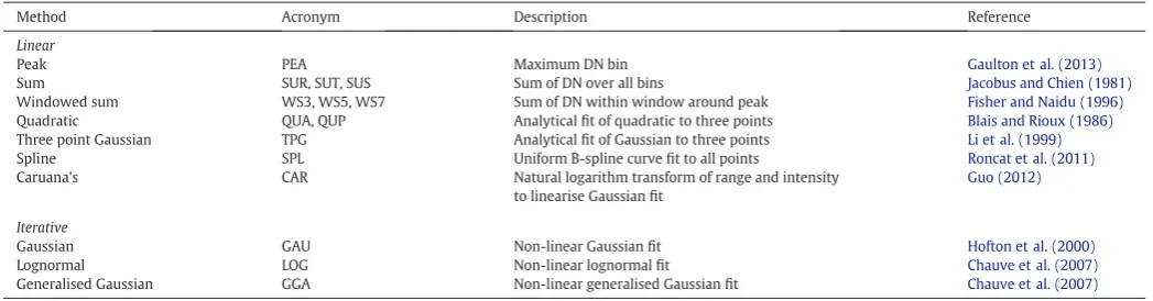
[image:7.595.41.565.76.213.2]

Some lidar algorithms assume that a return comes from a single in-teraction (such as the peak method). This is valid for hard targets, such as rocks and buildings, but is often not valid for vegetation, where the pulse can hit multiple targets through the canopy. It has been suggested that vegetation elements tend to be arranged as a Gaussian so that the Table 2

Waveform energy interpretation methods along with a reference for a paper using each.

Method Acronym Description Reference

Linear

Peak PEA Maximum DN bin Gaulton et al. (2013)

Sum SUR, SUT, SUS Sum of DN over all bins Jacobus and Chien (1981)

Windowed sum WS3, WS5, WS7 Sum of DN within window around peak Fisher and Naidu (1996)

Quadratic QUA, QUP Analyticalﬁt of quadratic to three points Blais and Rioux (1986)

Three point Gaussian TPG Analyticalﬁt of Gaussian to three points Li et al. (1999)

Spline SPL Uniform B-spline curveﬁt to all points Roncat et al. (2011)

Caruana's CAR Natural logarithm transform of range and intensity

to linearise Gaussianﬁt

Guo (2012)

Iterative

Gaussian GAU Non-linear Gaussianﬁt Hofton et al. (2000)

Lognormal LOG Non-linear lognormalﬁt Chauve et al. (2007)

(8)

returned waveform (convolution of the target and system pulse) can also be represented by a Gaussian (Hofton et al., 2000). If there are de-viations from these assumptions the methods that rely on them will struggle.

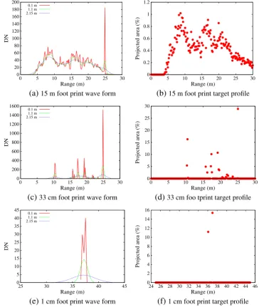
To test these assumptions the ray tracer ofLewis (1999)and the mixed age sitka spruce forest model described in Hancock et al. (2011)were used to generate waveforms. This tool has been widely used for simulating remote sensing measurements (Disney, Lewis, & Saich, 2006; Hancock, Lewis, Foster, Disney, & Muller, 2012), has been validated (Widlowski et al., 2007) and forms part of the RAMI surrogate truth (Widlowski et al., 2008). libRAT allows realistic lidar signals to be produced where the truth is known and so forms a virtual laboratory (Lewis, 1999). Three different footprint sizes were simulated, a very small footprint terrestrial system (1 cm at 10 m), a small footprint airborne system (33 cm) and a larger footprint air or spaceborne system (15 m). 15 m was chosen to lie between the spaceborne (GEDI at 25 m) and airborne (SLICER at 10 m) system footprints. For each footprint size three different pulse lengths were simulated,σ= 0.1 m,σ= 1.1 m and

σ= 2.15 m. Only a Gaussian system pulse was used to reduce compu-tational expense.

To ensure that a range of structures were covered at each pulse length, 25 waveforms were created for the 15 m footprints, 100 for

the 33 cm footprints and 283 for the 1 cm footprints. Different numbers were used because as footprint size increases more orders of multiple scattering and rays need to be simulated in order to achieve conver-gence in the Monte Carlo solution (Hancock, 2010, chapter 4), increas-ing the computational expense. In addition the target becomes more heterogeneous at smaller footprint sizes, so that more waveforms are needed to ensure that all possibilities are represented.

4.2.1. Return complexity

The measured waveforms and true target proﬁles visible to the in-strument were examined to see if the above assumptions about target arrangement were valid at the different footprint sizes. It was expected that the largest footprint's waveforms would most closely resemble a Gaussian (Hofton et al., 2000), whilst the smallest footprint would be more heterogeneous and less likely to contain returns from multiple targets.

4.2.2. Fitting to diffuse targets

The energy retrieval algorithms were then applied to these simu-lations using the noise removal method described inSection 3.3. Extracting the biophysical parameters or performing a classiﬁcation is beyond the scope of this paper and will be covered in a future study.

0 20 40 60 80 100 120 140

6 8 10 12 14

DN

Range (m)

0 20 40 60 80 100 120 140 160

6 8 10 12 14

DN

Range (m)

0 20 40 60 80 100 120 140

6 8 10 12 14

DN

Range (m)

(c)

n=3,

σ

= 0.1

m

0 20 40 60 80 100 120 140 160

6 8 10 12 14

DN

Range (m)

0 20 40 60 80 100 120 140 160

6 8 10 12 14

DN

Range (m)

0 20 40 60 80 100 120 140 160 180

6 8 10 12 14

DN

Range (m)

(e)

n=10,

σ

= 0.1

m

(f)

n=10,

σ

= 1.1

m

(d)

n=3,

σ

= 1.1

m

[image:8.595.118.468.52.482.2]

(a)

n=0,

σ

= 0.1

m

(b)

n=0,

σ

= 1.1

m

(9)

Here theﬁt was evaluated by the total energy returned and failure rate. The extractions were performed over the same range of noise levels (0_≤n_≤20 with_ﬁfty repetitions with different random number seeds for each waveform) as the single return experiments. The signals were smoothed by a range of Gaussians with widths between 0 (no smooth-ing) and 8 m.

Some of the methods rely on the identification of turning points in order to pick initial estimates (GAU, LOG and GGA) or to determine the number of individual features within a single return (GAU, LOG, GGA, PEA, WS3, WS5, WS7, QUA, QUP, TPG and CAR) and so could ben-efit from smoothing the data in order to identify these points, but not using the extra smoothing forfitting (Hofton et al., 2000). Therefore an additional“pre-smoothing”, separate to the smoothing mentioned above, was included. This was by a Gaussian between 0 (no smoothing) and 8 m long. To make sure that the accuracy was optimal for each method, only the accuracies for the smoothing combination with the lowest RMSE and a failure rate less than 2% were presented for each method. Smoothing was only used if it gave more than a 1% RMSE improvement above the unsmoothed accuracy. For the iterativefitting methods (GAU, LOG and GGA) the parameters were constrained within MINPACK. The position (μ) was forced to lie between the start and end of the feature, with the initial estimate at the centre of gravity. The amplitude (A) was forced to lie between twice and a quarter of the ob-served peak. The width (σ) was forced to lie between 0.00001 m and the total feature width. The additional parameters in the lognormal and generalised Gaussian were notfixed.

4.2.3. Processing time

In order to assess computational efﬁciency for realistic waveforms, the processing time for each method to estimate return energy from the diffuse target simulations was assessed. This was done within the C program by calling theclock() function before and after each method was performed to give the number of central processing unit, CPU, clock cycles. The CPU time was measured for each separate return along a waveform and the mean reported. Some of the related methods were calculated within the same function and so the measured time was for all sub-methods (the sums, windowed sums and quadratic). This may have slightly increased the reported time, but due to their similarity and common loops, this increase is negligible.

5. Results and discussion

5.1. Single returns

Results are presented separately for the unsmoothed raw data (Section 5.1.1) and smoothed (Section 5.1.2) cases.

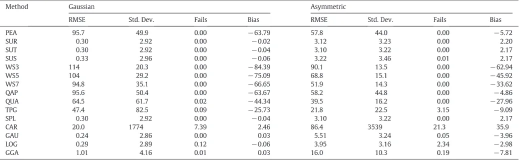
[image:9.595.43.569.584.744.2]

5.1.1. Unsmoothed raw data

Table 3shows the results for all methods at noise level 1 (the closest to the SALCA and Leica ALS50-II behaviour). Examining the standard deviation of return energies for a given pulse energy, the peak (PEA), windowed sums (WS3, WS5 and WS7), quadratic (QUA and QUP), three point Gaussian (TPG) and Caruana's (CAR) all gave unacceptably large errors. These occurred at all noise levels suggesting that they are not robust enough to be used on raw data. The sum using Simpson's rule (SUS) performed worse than both the rectangular sum and the tra-pezium sum and so was also rejected.

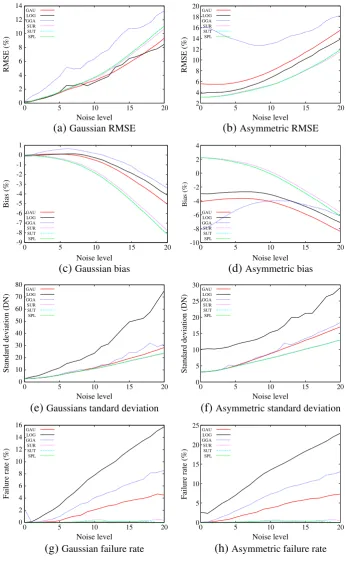
Fig. 7shows the four error metrics (mean across all pulse ampli-tudes, widths and ranges) against noise level for all feasible methods for Gaussian and asymmetric pulses. The lognormal method had higher errors at all noise levels, even for the asymmetric pulses it was intended for. This agrees with theﬁndings ofChauve et al. (2007)and was most likely due to the instability ofﬁtting a more complicated function.

For Gaussian pulses (Fig. 7), the five remaining methods gave near identical RMSEs and standard deviations for noise levels up to 8 (a high level), though the Gaussian gave a lower bias due to its ability to reconstruct the missing data. Above noise level 8 the generalised Gaussian started to give larger errors (due to numerical instability) whilst the Gaussian gave slightly larger standard deviations than the spline or two sum methods. The Gaussian gave slightly lower RMSEs (of the order of 0.5%) because of the lower bias. The generalised Gaussian and Gaussian started to fail tofit to some returns at noise levels of 3 and 5 respectively. The sum and spline showed negligible fail-ures up to the highest noise level tested. These three linear methods (SUR, SUT and SPL) are superior for Gaussian pulses due to their compu-tational efficiency and, at high noise levels, low standard deviations and failure rates. The differences between the performance of these three was negligible.

For asymmetric pulses (Fig. 7) again the lognormal showed higher errors due to instability. The otherfive methods gave near identical standard deviations until a noise level of 5 after which the spline, rect-angular sum and trapezium rule gave lower errors than the Gaussian and generalised Gaussian methods. The iterativefitting methods started to fail at lower noise levels than for Gaussian pulses (at noise level 2). Again the spline and sum methods showed negligible failures at all noise levels. Interestingly the spline and sum methods showed lower bias and RMSE than the iterative methods at all noise levels. This must be due to the deviation of the pulse shape (Fig. 3(b)) from a simple an-alytical form making function_fitting less robust. When successful the generalised Gaussian gave lower bias and RMSEs than the Gaussian due to its greater number of degrees of freedom, though this also caused more failures due to instability. It is concluded that the spline, rectangu-lar sum and trapezium rule gave more accurate results for asymmetric pulses in all conditions.

Table 3

Energy errors for simulations of single returns at noise level 1. All values are in %.

Method Gaussian Asymmetric

RMSE Std. Dev. Fails Bias RMSE Std. Dev. Fails Bias

PEA 95.7 49.9 0.00 −63.79 57.8 44.0 0.00 −5.72

SUR 0.30 2.92 0.00 −0.02 3.12 3.23 0.00 2.20

SUT 0.30 2.92 0.00 −0.04 3.10 3.22 0.00 2.17

SUS 0.33 2.96 0.00 −0.06 3.22 3.46 0.01 2.17

WS3 114 20.3 0.00 −84.39 90.1 13.5 0.00 −62.94

WS5 104 29.2 0.00 −75.09 68.8 15.1 0.00 −45.92

WS7 94.8 35.1 0.00 −66.65 51.9 14.3 0.00 −33.62

QAP 95.6 50.4 0.00 −63.67 58.2 44.8 0.00 −4.86

QUA 64.5 61.7 0.02 −44.34 39.5 16.2 0.00 −27.96

TPG 47.4 82.5 0.09 −25.73 21.8 22.5 3.15 −9.09

SPL 0.30 2.92 0.00 −0.04 3.10 3.22 0.00 2.17

CAR 20.0 1774 7.39 2.46 86.4 3539 21.3 35.9

GAU 0.24 2.86 0.00 0.03 5.51 3.24 0.05 −3.96

LOG 0.29 2.89 0.12 −0.06 3.95 3.16 2.34 −2.98

(10)

Examining the dependence of errors on amplitude and pulse width revealed that all the feasible methods gave higher errors for the very shortest (_σ_b0.2 m) and lowest amplitude (A_b50) returns. They all per-formed equally badly for these hardest cases and gave low errors for the shortest pulses if the amplitude was greater than 50 and for low ampli-tude returns if width was greater than 0.2 m. Therefore SALCA's very short pulse width was only an issue for low amplitude returns (RMSEs of 17% forDNb10 above noise). The RMSE could be reduced to 10% by doubling the sampling rate. This suggests that using a system pulse

longer than 0.2 m sampled at 1 ns would ensure that energy accuracy is not limited for single returns.

It is concluded that the spline, rectangular sum and trapezium rule were the most accurate methods for extracting return energy from raw lidar waveforms. They are far less computationally expensive than the iterativeﬁtting methods, more robust (lower failure rate) and gave more accurate results for asymmetric pulses and for Gaussian pulses at higher noise levels (ngreater than 6). At the low noise levels shown by SALCA and the Leica ALS50-II, the Gaussian method had a

0 2 4 6 8 10 12 14

Asymmetric failure rate

(11)

very slightly lower RMSE and bias (0.06% difference) for Gaussian pulses, but this came at the cost of extra computational expense and larger errors at higher noise levels.

5.1.2. Smoothed data

The analysis was repeated after smoothing by a 1.5 m long Gaussian and these are shown inTable 4for noise level 1. All methods, except Caruana's, gave acceptable standard deviations and negligible failure rates. The RMSEs for the methods that performed well without smooth-ing were slightly larger after smoothsmooth-ing due to an increased bias. This may have been due to signal being smoothed beneath the noise thresh-old and this supports the argument for using raw data (Press et al., 1994).

Smoothing caused a drop in the standard deviation of the peak, win-dowed sums, quadratic and three point Gaussian methods, all of which gave acceptable results. The quadratic method (QUA) now gave the lowest standard deviation for a Gaussian pulse, though the RMSE and

bias were much higher than for the other methods. For an asymmetric pulse, the windowed sum over three bins (WS3) gave the lowest stan-dard deviation (0.81%) followed by the windowed sum overﬁve (WS5, 1.39%) then the peak and quadratic (PEA, QUA 1.48%) methods. It is not clear why the standard deviation for the asymmetric pulse was lower than for the Gaussian pulses, other than possibly due to a difference in deﬁnitions of pulse width (σfor an asymmetric pulse is not directly comparable toσfor a Gaussian).

[image:11.595.43.563.76.236.2]

Fig. 8shows the standard deviations and RMSEs of extracted DNs against noise level using a smoothed waveform. After smoothing, the quadratic method gave the lowest errors at low noise levels for Gaussian pulses and the three bin windowed sum gave the lowest errors at high noise levels and for asymmetric pulses, closely followed by the peak method. This must be due to smoothing's ability toﬁll in the gaps be-tween samples by taking local averages and the suppression of noise. The three point Gaussian method showed a similar noise dependence to the quadratic method (they are mathematically very similar) but Table 4

Energy errors for noise level 1 after smoothing waveforms by a 1.5 m Gaussian. All values are in %.

Method Gaussian Asymmetric

RMSE Std. Dev. Fails Bias RMSE Std. Dev. Fails Bias

PEA 107 6.85 0.00 −80.55 98.6 1.43 0.00 −75.13

SUR 0.52 3.23 0.00 0.20 3.81 3.53 0.00 2.90

SUT 0.52 3.23 0.00 0.20 3.81 3.53 0.00 2.90

SUS 0.52 3.23 0.00 0.20 3.81 3.53 0.00 2.90

WS3 120 3.71 0.00 −91.54 117 0.81 0.00 −90.13

WS5 113 6.16 0.00 −85.96 107 1.39 0.00 −83.66

WS7 106 8.55 0.00 −80.46 98.5 1.97 0.00 −77.34

QAP 107 6.85 0.00 −80.55 98.5 1.43 0.00 −75.12

QUA 32.2 2.18 0.00 −24.67 30.8 2.48 0.00 −23.44

TPG 3.81 5.18 0.00 2.60 5.54 3.90 0.00 4.15

SPL 0.52 3.23 0.00 0.20 3.81 3.53 0.00 2.90

CAR 6.30 22.9 0.31 1.50 23.4 30.0 1.67 8.61

GAU 0.33 2.97 0.00 0.06 3.04 3.31 0.00 2.20

LOG 0.34 2.96 0.01 −0.05 3.07 3.33 0.08 2.20

GGA 0.71 3.62 0.19 −0.12 2.97 3.91 0.66 1.87

0 5 10 15 20 25 30

Asymmetric pulse

(12)

with a consistently higher error. The Gaussian and general Gaussian

ﬁttings performed similarly with and without smoothing (though smoothing reduces failures) whilst the spline and sum methods showed higher errors than without smoothing (due to bias).

5.1.3. Single return conclusions

The results show that for Gaussian pulses the most accurate methods (lowest RMSE with the lowest failure rate) were the Gaussian (GAU), sum (SUR) and spline (SPL) without smoothing whilst for asym-metric pulses the most accurate were the spline (SPL) and sum (SUR and SUT) without smoothing. As the sum and spline gave the joint low-est errors no matter the pulse shape and did not fail at higher noise levels, it is concluded that these are the most appropriate methods for determining lidar return intensity.

After smoothing, the windowed sum (WS3), peak (PEA) and qua-dratic (QUA and QUP) methods gave the most consistent results (lowest standard deviation) and so can be calibrated to get accurate reﬂectance, closely followed by the sum (SUR, SUT and SUS) and three point Gauss-ian (TPG). However, these assume that the peak is related to the total energy in the pulse. This is the case as long as the return is from a single object but not if from multiple objects. This is tested inSection 5.2.

Smoothing reduced the failure rate of iterativeﬁttings but did not in-crease accuracy.

5.2. Diffuse targets

Results for processing waveforms from diffuse targets are presented separately for target complexity (Section 5.2.1), ﬁtting accuracy (Section 5.2.2) and computational processing time (Section 5.2.3).

5.2.1. Return complexity

Fig. 9shows some typical simulated waveforms of sitka spruce for-ests at the three footprint sizes and three pulse lengths along with the target pro_ﬁles (the waveform without any pulse shape or sampling effects). The 15 m and 33 cm footprints were looking down from above whilst the 1 cm footprints were looking up at the canopy. It can be seen that the waveforms became more complex as the footprint size increased due to more canopy elements being illuminated.

In the 15 m footprint (Fig. 9(a)) many elements blurred together to form a continuous waveform. For the 1.1 m and 2.15 m pulses this re-sembled a Gaussian, but the target proﬁle (Fig. 9(b)) shows that this was a result of the system pulse. Therefore whilst a Gaussian (or lognor-mal or generalised Gaussian) could beﬁtted, the assumption that this

0 20 40 60 80 100 120 140 160 180 200

1 cm foot print wave form

0 2 4 6 8 10 12 14 16

24 26 28 30 32 34 36 38 40 42 44 46

Projected area (%)

Range (m)

[image:12.595.109.474.296.728.2]

(f)

1 cm foot print target profile

(13)

will retrieve the true target proﬁle may not be valid. Note that this in-cludes no noise so allﬂuctuations are due to heterogeneity. The wave-form was less complex for a 33 cm footprint but there were still areas with multiple returns combined into a single feature and so deviating from a simple analytical form. For the 1 cm footprint there were far fewer features with returns from multiple elements and so the assump-tion of single hits was more appropriate than for the larger footprints, but was not true in all cases.

If a return feature was more than one bin wide (1 ns) there were multiple elements contributing and so the assumption that the peak in-tensity is related to energy is not appropriate. For the 15 m footprint simulations there were no returns from single bins and for 33 cm foot-prints only 22% of returns came from single bins, the rest coming from more complex shapes. For 1 cm footprints all returns were from a single bin. To see whether these returns within a bin came from a single or multiple interaction the ray tracing simulations were repeated at 2 cm resolution and the number of separate returns within each 15 cm bin were added up. This showed that for 15 m footprints, only 1.3% of bins contained returns from single objects, for 33 cm footprints 20.6% and for 1 cm footprints 40.8%. Therefore at all footprint sizes the majority of returns over vegetation were complex and so we argue that the methods that assume single returns are not appropriate (the peak, win-dowed sum and quadratic).

5.2.2. Fitting to diffuse targets

The results forfitting to 15 m footprints are shown inTable 5. Only the results for noise levels 1 (as for SALCA and the Leica ALS50-II) and 10 (a high noise level) are shown as these show the overall behaviour at other noise levels. The standard deviation for the methods that mea-sure peak intensity rather than an integral of energy (PEA and QUP) was examined and found to have larger errors than the standard deviations for other methods (such as GAU and SUR) and so these could not be re-liably calibrated back to true intensity. The methods behaved similarly to thefits to single returns, with several giving unusable results in all cases no matter what smoothing was applied (CAR, QUP, QUA, WS3, PEA and TPG). The windowed sum (WS7 and WS5) seemed to perform well, but this was found to only be the case for low smoothing widths, where smallfluctuations in signal would cause many turning points, each of which was picked up as a separate feature. The low RMSE is a re-sult of a particular smoothing width leading to just enough features to add up all the energy, making them equivalent to SUR. The accuracy was unstable with changing smoothing widths and noise levels and so this is not a practical way to overcome bias. The LOG and GGA methods had low accuracies due to instability. The Gaussian, spline and sum methods all behaved similarly, with no more than 2% difference in accu-racy. At low noise levels (n = 1) or long pulse lengths (σ= 2.15 m)

Gaussianﬁtting gave slightly (0.5% difference) lower errors whilst the sum and spline performed better (1% difference) in other situations.

Gaussianﬁtting required the maximum smoothing (8 m smooth and 8 m pre-smoothing for parameter selection) whilst the sum and the spline required none. Smoothing by a 5 m Gaussian was found to re-duce the sum and spline RMSEs by 0.1% due to a change in the bias, as more signal was put beneath the noise threshold, but this small increase was not thought to be worth the additional computational expense. The errors reduced with shorter pulses, which is not what would be expect-ed from the rexpect-educexpect-ed information content (Landi, 2002). This was be-cause these diffuse target proﬁles (as inFig. 9(a)) meant that enough information was available for even the shortest pulse. This has implica-tions for sensor design.

For 33 cm footprints (Table 6) again some methods did not give ac-curate results (PEA, QUP, QUA, TPG, CAR, LOG and GGA). The windowed sum (WS3) appeared to be the best for short pulses but again this was an artefact due to noisefluctuations in the signal. Gaussianfitting, the sum and the spline were the most accurate methods (SUS was more sensitive to noise than SUR and SUT). The sum (SUR and SUT) and the spline gave almost identical accuracies. The trapezium rule (SUT) per-formed better than the simple sum (SUR) for short pulse lengths, due to there being more missing data tofill in, whilst SUR performed better for longer pulses. The spline had near identical accuracies to the trape-zium rule (SUT). Accuracies for all methods increased with longer pulses, as we would expect from the increased information content (Landi, 2002). It appears that at this footprint size the target pro_file is not extended enough to allow a short pulse to measure as accurately as a longer pulsed system.

Again the sum and spline required no smoothing. The smaller foot-print gave rise to a less diffuse target proﬁle (Fig. 9(c)) which did not show the same relationship between smoothing width and bias evident in the 15 m footprints. The Gaussian performed best after the longest smoothing widths (8 m).

The methods showed the same relative behaviour for the 1 cm foot-prints (Table 7) as for the 33 cm footprints (Table 6), though with higher errors and an increased sensitivity to noise at the shortest pulse length (σ= 0.1 m). The sum and spline performed better than the Gaussian in all situations and were less sensitive to noise (except for SUS which was unstable). Again the sum and spline required no smoothing whilst Gaussianﬁtting needed the maximum smoothing (8 m).

It is concluded that the spline (SPL) and rectangular sum (SUR as it gave near identical results but is simpler than SUT) were the most ap-propriate for extracting return energies from waveform lidar over veg-etation, except for large footprint (15 m) systems, where Gaussian

[image:13.595.309.560.583.745.2]

ﬁtting gave a 1% lower RMSE. The results for smaller footprints (33 cm and 1 cm) back up the observation ofJacobus and Chien (1981)that

Table 5

Mean relative RMSEs for extractions from simulated 15 m footprint waveforms using op-timal smoothing values for each method. All errors are in %.

Pulse method

0.1 m 1.1 m 2.15 m

n = 1 n = 10 n = 1 n = 10 n = 1 n = 10

PEA 36.4 30.2 85.0 84.6 89.8 89.4

SUR 6.51 10.3 12.7 12.8 12.8 12.9

SUT 6.54 10.3 12.7 12.9 12.8 12.9

SUS 6.04 10.3 12.7 12.9 12.8 12.9

WS3 32.6 39.8 71.6 39.1 80.2 35.0

WS5 15.8 34.0 57.4 24.6 73.3 21.7

WS7 9.22 32.9 46.1 18.2 68.0 16.8

QUP 80.7 78.6 NA 93.6 NA NA

QUA 28.5 185.3 31.5 44.2 NA 36.0

TPG 99.6 100.1 NA NA NA NA

SPL 6.53 10.3 12.7 12.9 12.8 12.9

CAR NA NA NA NA NA NA

GAU 5.71 12.1 12.2 11.8 12.3 12.0

LOG 96.3 96.4 72.4 89.2 69.7 NA

GGA 23.0 21.3 35.9 23.6 36.5 NA

Table 6

Mean relative RMSEs for extractions from simulated 33 cm footprint waveforms using op-timal smoothing values for each method. All errors are in %.

Pulse method

0.1 m 1.1 m 2.15 m

n = 1 n = 10 n = 1 n = 10 n = 1 n = 10

PEA 93.3 81.2 42.0 41.6 62.5 60.1

SUR 9.65 11.7 0.57 6.93 1.31 3.90

SUT 7.90 11.6 0.56 7.28 1.32 4.01

SUS 11.6 16.1 0.57 7.35 1.32 4.04

WS3 6.05 15.2 55.2 49.7 82.3 44.4

WS5 7.08 13.8 33.8 30.4 72.8 30.9

WS7 7.53 13.6 20.1 18.7 64.1 22.8

QUP 95.3 86.7 65.8 55.2 83.1 49.5

QUA 85.4 54.5 30.4 216.6 26.2 84.9

TPG 94.0 88.8 87.4 80.8 100.2 100.2

SPL 7.90 11.6 0.56 7.29 1.32 4.01

GAU 11.2 41.2 1.37 13.0 1.40 4.71

LOG 104.1 58.6 94.2 92.7 89.9 92.6

[image:13.595.43.296.583.743.2]

(14)

assuming an expected waveform shape will hide any deviations from it, potentially reducing the accuracy. This is especially true over vegetation where complex shapes can arise that do notﬁt simple models, such as the shadowed ground return under heterogeneous canopies (Hancock et al., 2012).

5.2.3. Processing time

The processing times are given inTable 8. The peak method was the fastest (as we would expect), closely followed by the sum, windowed sums, then the quadratic, three point Gaussian, spline andﬁnally the three iterative methods were several orders of magnitude slower; 1000 times slower for a 1.1 m pulse and 33 cm footprints and 20,000 times slower for 2.15 m pulses and 33 cm footprints. This supports the previous claims that iterativeﬁtting methods are the most computa-tionally expensive (Neuenschwander et al., 2009) which may limit their applicability to large datasets (Jalobeanu & Gonçalves, 2014). Pro-cessing time increased with large footprints and longer system pulses due to the larger volume of data, even for the methods that use a subset of the data, as they still need to search through the larger data volume to identify the points of interest. The different processing times for the grouped methods (the quadratic and sum methods) were due to differ-ent optimal smoothing widths.

Examination of the contribution of smoothing to the computa-tional expense shows that TPG would have been the fastest method in the absence of smoothing and so may be the most computationally efficient method when using thefiltering proposed byJalobeanu and Gonçalves (2014). For the iterativefitting methods (GAU, LOG and

GGA) around 50% of the processing time was due to smoothing and so they would still be much slower with more efﬁcient ﬁltering methods. The windowed sums were faster than the sum but required more smoothing, slowing them down. The sum and spline required no smoothing.

5.2.4. Diffuse target conclusions

Due to broadening of returns by diffuse targets it cannot be assumed that the peak intensity is related to energy and so the peak, quadratic and windowed sum methods, which performed well for single returns after smoothing, were deemed unsuitable. The three point Gaussian gave reasonable estimates for small footprints, where returns are likely to be narrow, but gave inaccurate energies for large footprints as the brightest three points did not fully describe the feature. Caruana's meth-od was as unstable for diffuse returns as for single returns and so was deemed unsuitable for analysing vegetation with waveform lidar. Vege-tation presents complex targets that are not perfectly modelled by sim-ple analytical forms. For large footprints (15 m) the target proﬁle approaches a collection of Gaussians and, after smoothing, Gaussian

ﬁtting gave the most accurate results (around 1% better than SUR, SUR and SPL). In all other cases the sum (SUR and SUT) and spline (SPL) were slightly more accurate (around 1% RMSE better) and have the ad-vantage of not needing any smoothing (maximising the resolution) and being far less computationally expensive.

Gaussianfitting is the most widely used method for interpreting waveform lidar, but these results show that equally accurate results can be achieved at a fraction of the computational expense by the sum and spline methods (around 1000 times faster for the sum and 15 times faster for the spline). Functionfitting (GAU, GGA, LOG and SPL after deconvolution) gives easily understandable metrics (location, en-ergy and width for each feature) that can be used for classifying vegeta-tion (Mallet et al., 2011; Roncat, Briese, Jansa, & Pfeifer, 2014). However these can also be derived from turning points in the waveform when using the sum and this identification of turning points, peaks and widths is a necessary step in order to choose initial estimates required for func-tion_fitting. Alternatively deconvolution could be used to retrieve the target profile (Hancock et al., 2008; Roncat et al., 2014). The relative ac-curacies of the resulting metrics (location and width) need to be assessed and will form a future investigation, but for return energy (and so target reflectance) these conclusions will still hold and it is pos-sible to use different algorithms for range and energy.

[image:14.595.35.286.85.245.2]

For large footprints (15 m) the accuracy was insensitive to noise and pulse length. For smaller footprints (33 cm) there was a strong relation-ship between pulse length, noise and retrieval accuracy. The longer the pulse the more accurate and less sensitive to noise the retrieval was. This has implications for sensor design. The results suggest that for a system with a noise level similar to SALCA or a Leica ALS50-II (n = 1),

Table 8

Mean processing time for a single return, in milliseconds, for the different methods at noise level 1, including any smoothing. NA indicates thatﬁt errors were not acceptable.

Footprint pulse

15 m 33 cm 1 cm

0.1 m 1.1 m 2.15 m 0.1 m 1.1 m 2.15 m 0.1 m 1.1 m 2.15 m

PEA 0.008 0.005 0.006 0.001 0.001 0.003 0.001 0.001 0.001

SUR 0.007 0.008 0.010 0.001 0.003 0.005 0.001 0.002 0.003

SUT 0.007 0.008 0.010 0.001 0.003 0.005 0.001 0.002 0.003

SUS 2.58 0.008 0.010 0.001 0.003 0.005 0.001 0.002 0.003

WS3 0.025 0.016 0.017 0.002 0.004 0.008 0.002 0.002 0.002

WS5 0.025 0.016 0.017 0.002 0.004 0.008 0.002 0.002 0.002

WS7 0.025 0.016 0.017 0.002 0.004 0.008 0.002 0.002 0.002

QUP 0.037 NA NA 0.003 0.008 0.012 0.002 0.003 0.004

QUA 2.56 2.54 NA 0.003 0.008 0.013 0.002 0.003 0.004

TPG 0.006 NA NA 0.020 0.024 0.021 0.016 0.010 0.015

SPL 1.48 1.82 2.22 0.043 0.26 0.76 0.040 0.14 0.35

CAR NA NA NA 0.004 NA NA 0.003 0.004 0.005

GAU 5.27 5.01 5.31 0.59 3.65 54.8 0.33 0.80 1.51

LOG 126 112 111 125 166 542 4.72 8.93 15.9

[image:14.595.36.552.583.744.2]

GGA 6.60 5.77 5.76 0.46 1.68 4.11 0.35 0.73 0.87

Table 7

Mean relative RMSEs for extractions from simulated 1 cm footprint waveforms using op-timal smoothing values for each method. All errors are in %.

Pulse method

0.1 m 1.1 m 2.15 m

n = 1 n = 10 n = 1 n = 10 n = 1 n = 10

PEA 105.7 68.9 87.4 87.5 53.3 51.0

SUR 10.8 19.9 0.48 4.00 0.22 2.04

SUT 9.13 22.1 0.43 4.01 0.22 2.03

SUS 15.8 42.4 0.45 4.25 0.25 2.14

WS3 8.32 33.0 55.5 53.9 95.5 57.3

WS5 8.58 33.6 28.1 26.9 83.2 41.7

WS7 8.61 33.8 12.3 11.4 71.5 30.9

QUP 108.6 82.3 31.3 34.6 75.2 50.2

QUA 23.8 31.6 28.4 33.1 28.3 29.2

TPG 24.9 71.0 3.55 31.3 2.66 5.18

SPL 13.9 24.2 0.44 4.16 0.23 2.06

GAU 14.4 40.2 2.16 7.88 1.22 5.52

LOG 18.5 41.5 5.80 9.96 6.86 4.35

(15)

a 2.15 m pulse sampled every 1 ns (or 1.1 m pulse sampled every 0.5 ns) would give a 2.7% error compared to a 3.4% error for a 1.1 m (0.6 m) pulse.

6. Conclusions

A range of methods for extracting return energy (and so reﬂectance) from waveform lidar have been tested on a range of targets and system parameters. As far as the authors are aware this included every method currently proposed for measuring waveform lidar energy and the full range of current and proposed full waveform lidar systems. The targets ranged from single returns to complex returns over vegetation and so this is theﬁrst time such an exhaustive cross-comparison has been car-ried out. Photon counting systems were excluded due to the repeat measurements needed to estimate energy.

For single returns the peak, quadratic and windowed sum methods gave the most consistent results after smoothing and so could easily be calibrated to give accurate energy from hard surfaces. However, this requires the peak intensity to be related to the total waveform en-ergy, an assumption that has been shown not to hold over vegetation and so these methods (and the three point Gaussian, which gave rea-sonable results) are deemed unsuitable. Caruana's method was too un-stable to provide accurateﬁts in all cases tested. This leaves the sum, spline and three iterativeﬁtting methods (SUR, SUT, SPL, GAU, LOG and GGA).

It has been shown that vegetation causes complex returns. For large footprints (15 m) these approached a Gaussian after smoothing so that Gaussianfitting (GAU) gave the most accurate results (around 1% lower RMSE than the sum and spline). For smaller footprints (33 cm and 1 cm) the sum (SUR and SUT) and spline (SPL) gave slightly more accurate (around 1% lower RMSE than Gaussianfitting). The sum and spline have the advantage of being robust, computationally efficient (the sum several hundred times more so than the spline) and making no as-sumptions about the target shape. Some interpretation will be needed to identify the location and distribution of individual targets, especially when the system pulse causes their waveforms to overlap. This can be achieved by functionfitting (Hofton et al., 2000), by examining turning points, which is a necessary step to choose initial estimates for function

ﬁtting or by deconvolution (Hancock et al., 2008; Roncat et al., 2014). An assessment of the relative accuracies of these will form a future paper. For small footprints (33 cm) there was a strong dependence of accuracy on system pulse length, with long pulses giving lower errors and being less sensitive to noise. This agrees with theﬁndings ofLandi (2002). Therefore there is a trade-off between energy accuracy, and the minimum separation that targets can be distinguished (for longer system pulses) or data volume (for higher sampling rates). This depen-dence disappears for large footprints (15 m) due to decreased target heterogeneity at this scale. This is good news for the proposed space-borne missions.

These results suggest that the spline and sum will give as good if not better results at a fraction of the computational expense, except for large footprint systems (15 m), where Gaussianﬁtting is marginally more accurate.

Datasets from some lidar instruments, such as the Riegl LMS-Q680i (footprint around 30 cm), were only available to some past studies in the form of Gaussianfit parameters due to proprietaryfile formats for waveform lidar data (Armston et al., 2013). Discrete return systems only report an energy derived from a proprietary algorithm, which also imposes additional restrictions on quantitative use of these data and may suffer from similar limitations. The results from this study show that these methods may limit the accuracy of retrieved lidar ener-gy over vegetation. New, open source,file formats are making full wave-form data more common (Bunting, Armston, Lucas, & Clewley, 2013). Thesefindings have implications for all full waveform lidar vegetation missions, such as JAXA's proposed Multi-Footprint Observation LiDAR

and Imager (MOLI) (Murooka et al., 2013) and NASA's recently funded Global Ecosystem Dynamics Investigation (GEDI) missions.

Acknowledgements

This work was funded by the NERC new investigator grant NE/ K000071/1 (PI R. Gaulton) and the NERC Biodiversity and EcoSystem Services (BESS-F3UES) project (PIs K. Anderson and K. Gaston). The experiment comparing DWEL, SALCA and the Reigl VZ-400 behaviour was under the umbrella of the terrestrial laser scanner international interest group, TLSIIG (http://tlsiig.bu.edu/). Thanks to the Douglas Bomford Trust for funding S. Hancock's involvement in the TLSIIG inter-comparison experiment that contributed to this work. Participa-tion by authors Z. Li and A. Strahler was supported by US NaParticipa-tional Sci-ence Foundation grant MRI-0923389. The Leica ALS50-II data were collected by the NERC Airborne Research and Survey Facility (ARSF) and were provided to K. Anderson under the NERC BESS-F3UES grant. We are particularly grateful to Drs. Mike Grant and Gary Llewellyn for their assistance with the NERC Leica ALS data. Thanks to the two anon-ymous referees for the thorough reviews.

Appendix A. Linear method descriptions

A.1. Peak (PEA)

This is the simplest method, with the brightest bin in a feature taken as the return energy. This is the value used byGaulton et al. (2013)for single leaves and the most closely correlated to the discrete return Leica ALS50-II output, though the exact algorithm used by Leica is proprie-tary. The disadvantage is it makes no attempt to reconstruct the missing data and ignores the effect of pulse broadening by diffuse targets. For short pulses (such asFig. 2(b)) this will lead to a change in measured energy as sub-bin range changes.

A.2. Sum (SUR, SUT, SUS)

This is the second simplest method, with the sum of the waveform values above a threshold taken as the energy (Jacobus & Chien, 1981; Landi, 2002). There are three variations of the sum method. The rectan-gular sum (SUR) adds up all bins above noise, making no attempt to re-construct missing data. Using the trapezium rule (SUT) or Simpson's rule (SUS) goes some way to trying to_ﬁll in the missing data (Stroud & Booth, 2003). This is also referred to as the“area under the curve” method. Range can be calculated from the similar“centre of gravity” (Jutzi & Stilla, 2005).

A.3. Windowed sum (WS3, WS5, WS7)

This is the same as the rectangular sum but only uses points within a defined number of bins from the peak to help avoid noise and reduce computational expense.Fisher and Naidu (1996)tested three (WS3, one bin either-side),five (WS5, two bins either-side) and seven (WS7, three bins either-side) point windows. This does not attempt tofill in missing data and assumes that the windowed areas describe the full re-turn.Jupp et al. (2009)used the mean of the brightest three bins, which is equivalent to WS3 but then applied a linear correction based on the sub-bin range. Thisfills in the gaps between datapoints but still assumes that the brightest three bins are representative of the whole return.

A.4. Quadratic (QUA, QUP)

A lidar pulse can be approximated as a quadratic function (Blais & Rioux, 1986; Jupp et al., 2009):