Comparative Thermal Analysis of Bar Element Connected to Different Heating Sources

(1)

International Journal of Emerging Technology and Advanced Engineering

Website: www.ijetae.com (ISSN 2250-2459,ISO 9001:2008 Certified Journal, Volume 4, Issue 12, December 2014)

72

Comparative Thermal Analysis of Bar Element Connected to

Different Heating Sources

Sampath S S

1

, Anil Antony Sequeira

2

, Chithirai Pon Selvan M

3

, Sawan Shetty

4 1, 2, 4

Assistant Professor – Senior Grade, Manipal University, Dubai, UAE

3_{Assistant Professor – Selection Grade, Manipal University, Dubai, UAE} Abstract—The present study investigates the temperature

distribution in a bar element which is connected to two different heat reservoirs. Over performance of the connecting element is improved by the selection of appropriate material which dissipates maximum rate of heat. An improvement in the performance is achieved by using the computational analysis software ANSYS CFX and the comparative tool software DOT NET. Various materials are considered for the bar element and the variation in the temperature distribution within the element are discussed.

Keywords—ANSYS CFX, DOT NET, Fin Geometry, Temperature Sources, Thermal analysis.

I. INTRODUCTION

According to the Kelvin Planck and Clausius statement of second law of thermodynamics heat always flow from a region of higher potential to the lower potential. This study involves the optimum material selection with a specific value of conductivity, in order to dissipate maximum heat to the sink. The modes of heat transfer involves conduction where heat flow within the material or same medium and convection where the heat flows from one medium to that of the other. Free convection takes place naturally and the forced convection occurs with the aid of external means. As experimented by Nagarani [1], an extended surface or a fin is provided to facilitate the heat transfer. There are various types of extended surfaces like infinitely long, short type, insulated type, connected fins etc.

The present study is involves a study of the heat transfer in the bar element connected to two different temperature sources [6]. Bar element which connects the sources are assumed to be a fin and conventional or theoretical equations of fin are used and a code is generated using the software DOT NET. The temperature distribution, fin factor, heat transfer rate are calculated. Various materials are considered and the heat transfer rate for the fixed convective coefficient value is calculated [1, 2]. Dot NET software gives flexibility to vary the conductivity and the optimum material selection [1] can be performed. In the present case a bar with circular cross section of diameter 15 mm and length 3 m is taken and the two different temperature sources are fixed to 300⁰C and 100⁰C.

Heat transfer coefficient value is fixed to 15 W/m2⁰C. The following element is modelled, meshed and analysed in dedicated software ANSYS CFX and the results and compared. Finite element approach provides the solution at every node of consideration [5].

This work was structured as a sequence of fundamental problems built on simple models that capture the most basic characteristics of the temperature distribution in a structure [3]. The models proceed from the simple toward the complex. The objective is to uncover the most fundamental optimization principles (or design trade-offs) that can be put to practical use in real applications. The method of analysis and optimization is the combination of heat transfer, thermodynamics and structures which is used subsequently in many engineering applications.

II. METHODOLOGY

In the present study the governing equations of heat transfer between the elements are applied. Below equation (1) represents the heat transfer which takes place during conduction derived by the Fourier, and equation (2) represents the heat transfer during conduction which is by Newton’s law of cooling [5]. The heat transfer from different heat sources that is different temperature [6] points is represented using equation (3). Temperature at any point in the element is determined by the equation (4).

Fourier’s Law of conduction

(1)

Newton’s Law of cooling

(2)

Heat transfer from different temperature sources

(2)

International Journal of Emerging Technology and Advanced Engineering

73

Temperature at any point in the element

(4)

Fin Factor

(5)

III. MODELLING AND ANALYSIS

In the current study geometric modelling of the heat transferring element is generated using ANSYS CFX and its simulation is performed using the same as conducted by Ashsh Giri[10]. The material of the element which is connected to the heat source is made up of copper with circular cross-section. The heating element with different temperatures is defined. Entire set up obeys the second law of thermodynamics which requires two reservoirs to transmit the heat. One reservoir will be the cylindrical element where the temperature is distributed and another is the atmosphere where the heat is dissipated. Different material can be chosen accordingly by changing the thermal conductivity of the material. The model of the heat sources and the element is shown in the figure 1 and the discretization of the cylindrical element is carried out using FEA software is shown in figure 2.

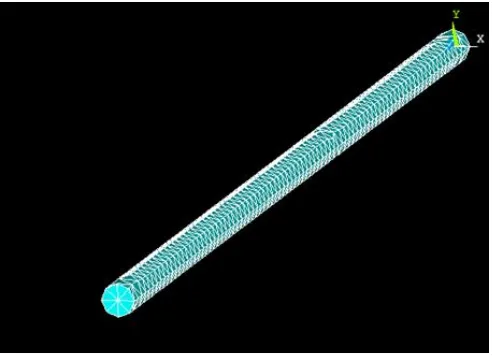
[image:2.612.325.569.135.315.2]

Heating element is modelled and it is meshed using ANSYS software. Meshing is discretizing of an element into finite number of parts and each element is considered and solved separately. Mesh generation is the practice of generating a polygonal or polyhedral mesh that approximates a geometric domain. The term "grid generation" is oftenly used interchangeably. Typical uses are for rendering to a computer screen or for physical simulation such as finite element analysis or computational fluid dynamics [4]. After this step a thermal steady state simulation is performed. By using ANSYS numerical simulation tool, whole analysis of entire assembly is performed. Present simulations adopt realistic boundary conditions by considering various different materials with different thermal conductivities.

[image:2.612.59.286.156.263.2]

Fig 1. Model of the cylindrical element connected to the heating sources

Fig 2. Meshing of the cylindrical element connected to the heating sources

Table 1.

Materials and their properties

Name Conductivity Heat Capacity

Copper 380 W/m⁰C 385 J/Kg ⁰C

Construction steel Fe 360 53 W/m⁰C 470 J/Kg ⁰C

Aluminium Alloy EN AW-1050 A

[image:2.612.324.570.348.526.2]

(3)

International Journal of Emerging Technology and Advanced Engineering

74

Due to high thermal conductivity and good machining properties, pure copper was considered as an ideal material. The second boundary in the simulation was the surface of the cylindrical element, where convection takes place. The value of film coefficient, especially when there is free convection for air is assumed to be 20 W/m2⁰C which lies within its limits. As an important boundary condition is the radiation property of the copper, due to the high film coefficient, the part of the heat flow caused by radiation is neglected in this work. Modelling and Meshing is done using FEA and the simulation is performed. By means of the numerical solution, a steady state analysis of the entire heating element is achieved. Validation of the results obtained in the FEA is carried out using Dot Net frame work software.

Dot Net provides user interface, data access, database connectivity, cryptography, web application development, numeric algorithms and network communications. Governing equations are fed and the results are obtained. Classical equations parameters are varied accordingly and the output relating to this are compared with the numerical method.

IV. RESULTS AND DISCUSSION

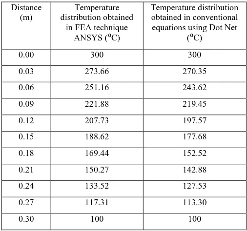
[image:3.612.324.571.246.391.2]

The simulation is carried out with the application of the boundary conditions by defining the temperatures at extreme ends of the cylindrical element. Conductivity and heat transfer coefficient are considered. Figure 3 shows the temperature distribution in the cylindrical element at various points. Table 2 shows the value of the temperatures obtained in both FEA and the conventional equations solved by Dot Net software.

Fig 3. Simulated result of the cylindrical element connected to two temperature sources

The above simulation in figure 3 shows the temperature distribution at various points of the cylindrical element. Temperature at the source 1 is maintained at 300⁰C and the temperature of the source 2 is at 100⁰C. There is a drastic drop in temperature from one end to the other is observed due to the effect of convection. Table 2 shows Temperature variation in temperature in the cylindrical element for fixed conduction and convection values by both FEA and the conventional equation.

[image:3.612.317.570.463.700.2]

Fig 4. Results obtained using Dot Net software

Table 2.

Temperature variation comparison

Constant Parameters:

K=380 W/m⁰C, h=20 W/m2_⁰_{C, Length of the element=0.3 m, diameter of}

the element = 0.015 m

Distance (m)

Temperature distribution obtained

in FEA technique ANSYS (⁰C)

Temperature distribution obtained in conventional equations using Dot Net

(⁰C)

0.00 300 300

0.03 273.66 270.35

0.06 251.16 243.62

0.09 221.88 219.45

0.12 207.73 197.57

0.15 188.62 177.68

0.18 169.44 152.52

0.21 150.27 142.88

0.24 133.52 127.53

0.27 117.31 113.30

[image:3.612.48.292.513.693.2]

(4)

International Journal of Emerging Technology and Advanced Engineering

75

Fig 5. Comparative temperature distribution using FEA and Classical methods

Figure 5 shows the graph which represents the temperature distribution in the element connected to different heat sources using both classical and FEA method. Results are almost matching with each other except at the middle of the element where there is a slight difference in the values observed.

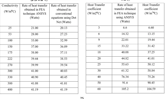
Table 3.

Thermal conductivity variation with the rate of heat transfer (h=20 W/m2⁰C)

Conductivity

(W/m⁰C)

Rate of heat transfer obtained in FEA technique ANSYS

(Watts)

Rate of heat transfer obtained in conventional equations using Dot

Net (Watts)

25 21.00 20.13

53 28.00 27.23

100 33.00 32.99

150 37.00 36.09

175 38.00 37.11

222 39.44 38.53

270 39.99 39.54

300 41.00 40.03

330 40.90 40.45

380 41.08 41.01

400 41.19 41.19

Figure 6 shows the graph which varies between heat transfer rate and thermal conductivity. Results are almost matching with each other except in the region where the thermal conductivity values lies between 200 W/m⁰C to 300 W/m⁰C.

[image:4.612.52.288.140.280.2]

Fig 6. Comparative Thermal Conductivity verses Heat transfer rate graph using FEA and Classical methods

Table 4.

Thermal conductivity variation with the rate of heat transfer (K=380 W/m⁰C)

Heat Transfer coefficient (W/m2⁰C)

Rate of heat transfer obtained in FEA technique using ANSYS

(Watts)

Heat Transfer coefficient

(W/m2⁰C)

3 6.6 6.60

6 14.32 13.15

9 22.01 19.44

15 33.22 31.42

18 40.08 37.25

20 44.82 41.01

25 55.63 50.12

30 61.32 58.84

40 76.34 75.26

50 91.6 90.45

[image:4.612.337.563.211.349.2] [image:4.612.43.572.412.730.2]

(5)

International Journal of Emerging Technology and Advanced Engineering

76

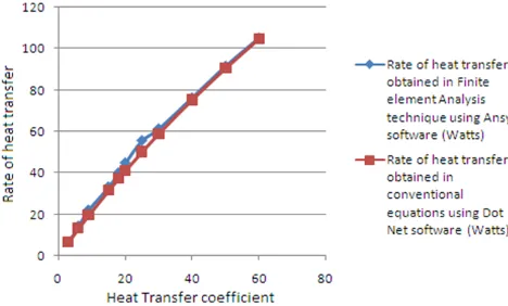
Figure 7 shows the graph which varies between heat transfer rate and Heat transfer coefficient. Results are almost matching with each other except in the region where the Heat transfer coefficient values lies between 20 W/m2⁰C to 30 W/m2⁰C.

[image:5.612.44.578.181.725.2]

Fig 7. Comparative Heat transfer coefficient verses Heat transfer rate graph using FEA and Classical methods

Table 5.

Thermal conductivity variation with the fin factor (h=20 W/m2_⁰_C)

Conductivity((W/m⁰C) Fin factor(m-1)

25 14.60

53 10.03

100 7.30

150 5.96

175 5.52

222 4.90

270 4.44

300 4.21

330 4.02

380 3.74

400 3.65

[image:5.612.327.568.196.327.2]

Figure 8 shows the graph which varies between thermal conductivity and fin factor. Results Shows that as the thermal conductivity of the material increases, fin property that is the fan factor decreases significantly.

[image:5.612.61.295.215.356.2]

Fig 8. Variation of Thermal conductivity with the Fin Factor

Table 6.

Thermal conductivity variation with the fin factor (K=380 W/m⁰C)

Heat transfer coefficient

(W/m2⁰C) Fin factor (m-1)

3 1.45

6 2.05

9 2.51

15 3.24

18 3.55

20 3.74

25 4.18

30 4.58

40 5.29

50 5.92

(6)

International Journal of Emerging Technology and Advanced Engineering

77

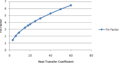
[image:6.612.56.295.200.325.2]

Figure 9 shows the graph which varies between heat transfer coefficient and fin factor. Results Shows that as the heat transfer coefficient of the material increases, fin property that is the fan factor increases significantly.

Fig 9. Variation of Heat transfer coefficient with the Fin Factor

V. CONCLUSIONS

In the present analysis, a fin or a cylindrical element connected to the different temperature source is investigated which enhances the temperature distribution and the heat dissipation from the entire unit. An attempt is made to demonstrate the improvements to enhance the maximum heat dissipation [6] from the system using FEA technique and the validation of this is carried out by using computer software Dot Net. It is possible to obtain an optimum solution by selecting a material which has better thermal performances. By increasing the value of thermal conductivity it is possible to increase the heat dissipation rate which is showed in the figure 5. Shape and size of the fin can also be varied to enhance the change in heat transfer. Concept of forced convection can also be implemented by providing external fan to dissipate the maximum heat transfer; calculations will required various dimensionless numbers like Nusselt, Prandtl and Reynolds numbers. Due to the forced convection the heat transfer will be transient and the effectiveness will be increased. Fin efficiency and effectiveness can be calculated using the equations and it could be varied in order to obtain an optimum values.

By providing multiple cylindrical elements or fins enhance the heat transfer which is undergoing forced convection. Surface area exposed will be greater than a single fin. In the present analysis, the convective ambience is affected in the form of boundary conditions. However better results could be obtained by simulating air around the fins.

Nomenclature

Q= Heat Transfer rate, W d= Diameter of the element, m Acs= Cross-Sectional Area, m2

K= Thermal Conductivity of the material, W/m⁰C h= Heat transfer coefficient, W/m2⁰C

T= Temperature, ⁰C As= Surface Area, m2 Ts= Surface Temperature, ⁰C Ta= Ambient Temperature, ⁰C x= length till the defined point, m p= Perimeter, m

m= fin factor, m-1

l= length of the element, m

θ1= temperature difference between temperature of source

1 with ambient temperature, ⁰C

θ2= temperature difference between temperature of source

2 with ambient temperature, ⁰C

θ= temperature difference between temperature at defined point on the fin with ambient temperature, ⁰C

REFERENCES

[1] N.Nagarani, “Experimental heat transfer analysis on Annular circular and elliptical fins” International Journal of Engineering Science and Technology, 2010, Vol. 2(7), PP: 2839-2845.

[2] Saeid. Rasouli, Mohammad.R. Golriz, “Effect of Fins on Heat Transfer of Horizontal Immersed Tube in Bubbling Fluidized Beds” World Congress on Engineering, 2009, Vol.II, PP: 1-4

[3] Amol B. Dhumne, Hemant S. Farkade, “Heat Transfer Analysis of Cylindrical Perforated Fins in Staggered Arrangement“ International Journal of Innovative Technology and Exploring Engineering (IJITEE),2013, Vol 2, PP: 225-230

[4] Dhanawade Hanamant S, K. N. Vijaykumar Dhanawade Kavita, “Natural convection heat transfer flow visualization of perforated fin arrays by CFD simulations” International Journal of Research in Engineering and Technology, 2013, PP: 483-490

[5] Esmail M.A. Mokheimer, “Performance of annular fins with different profiles subject to variable heat transfer coefficient” International Journal of Heat and Mass Transfer, 2002, PP: 3631-3642

[6] Pardeep Singh, Harvinder lal, Baljit Singh Ubhi, “Design and Analysis for Heat Transfer through Fin with Extensions”, International Journal of Innovative Research in Science Engineering and Technology, 2014, Vol.3, PP: 12054-12061

(7)

International Journal of Emerging Technology and Advanced Engineering

78

[8] Pankaj N. Shrirao, Rajeshkumar U.Sambhe, Pradip R.Bodade,” Convective Heat Transfer Analysis in a Circular Tube with Different Types of Internal Threads of constant Pitch”, International Journal of Engineering and Advanced Technology, 2013, Vol 2, PP 335-340 [9] Wadhah Hussein Abdul Razzaq Al- Doori, “Enhancement of Natural

convection heat transfer from the rectangular fins by circular perforations”, International Journal of Automotive and Mechanical Engineering, 2011, Vol 4, PP 428-436

[10] Ashish Giri, Evaluation of the Performance of Annular Composite Fin using ANSYS, International Journal of Computer Applications, 2012, Vol 44, PP 4-7