Eigenvalue regularized covariance matrix estimators for high dimensional data

(1)

Eigenvalue-Regularized Covariance

Matrix Estimators for

High-Dimensional Data

Huang Feng

Department of Statistics

London School of Economics and Political Science

A thesis submitted for the degree of

Doctor of Philosophy

(2)

致我最爱的家人

(3)

Declaration

I hereby declare that the thesis submitted for the PhD degree of the London School of Economics and Political Science is my own work except where specific reference is made to the work of others (in which case the extent of any work carried out jointly by me and any other person is clearly identified in it). This thesis has not previously been submitted in whole or in part for consideration for any other degree.

I confirm that Chapter3, 4 and 5are jointly co-authored with Dr. Clifford Lam.

(4)

Acknowledgements

First of all, I would like to thank my supervisor, Dr. Clifford Lam, for his immense support, inspiring guidance and invaluable encouragement throughout my PhD study. I am extremely lucky to have a supervisor who cares so much about my work. I could not ask for more from such a nice supervisor. I would also like to show my deep gratitude to my second supervisor, Professor Piotr Fryzlewicz, for his suggestion and recommendation for my pursue of PhD study.

I would like to express my great appreciation to all the staff and colleagues in the Department of Statistics at the LSE, for making the last four years a great experience. Special thanks to all my lovely officemates Andy Ho, Haziq Jamil, Tayfun Terzi, Yajing Zhu, Ragvir Sabharwal, Yan Qu, Xiaolin Zhu, Alice Pignatelli di Cerchiara and Filippo Pellegrino for helping me with my endless academic and non-academic questions and giving me great support for surviving the PhD. I wish to acknowledge the help provided by the students of my supervisor Charlie Hu and Cheng Qian for the efficient discussions about the research. I am particularly grateful for the invitation from Dr. Wicher Bergsma, Dr. Matteo Barigozzi and Dr. Yining Chen to be their teaching assistant, and same thanks to my teaching partner José Manuel Pedraza Ramirez for making wonderful teaching experience as a team. Assistance provided by Ian Marshall and Penny Montague was greatly appreciated. Besides, my research would not have been possible without the sponsorship from LSE.

(5)

Abstract

Covariance regularization is important when the dimension pof a covariance matrix is

close to or even larger than the sample size n. This thesis concerns estimating large

covariance matrix in both low and high frequency setting.

First, we introduce an integration covariance matrix estimator which is a linear combination of a rotation-equivariant and a regularized covariance matrix estimator that assumed a specific structure for true covariance Σ₀, under the practical scenario where one is not 100% certain of which regularization method to use. We estimate the weights in the linear combination and show that they asymptotically go to the true underlying weights. To generalize, we can put two regularized estimators into the linear combination, each assumes a specific structure for Σ0. Our estimated weights can then

be shown to go to the true weights too, and if one regularized estimator is converging to Σ0 in the spectral norm, the corresponding weight then tends to 1 and others tend

to 0 asymptotically. We demonstrate the performance of our estimator when compared to other state-of-the-art estimators through extensive simulation studies and a real data analysis.

Next, in high-frequency setting with non-synchronous trading and contamination of microstructure noise, we propose a Nonparametrically Eigenvalue-Regularized In-tegrated coVariance matrix Estimator (NERIVE) which does not assume specific structures for the underlying integrated covariance matrix. We show that NERIVE is positive definite in probability, with extreme eigenvalues shrunk nonlinearly under the high dimensional framework p/n→c >0. We also prove that in portfolio allocation,

the minimum variance optimal weight vector constructed using NERIVE has maximum exposure and actual risk upper bounds of order p−1/2. The practical performance of

(6)

vi

(7)

List of figures

3.1 Boxplot of the absolute forecast errorsEk,jin (3.16) for different methods

with 120 days training data. . . 58

4.1 Boxplot of Frobenius errors when there are no factors in model (4.14) (C = 0). . . 107

(11)

List of tables

3.1 Mean and standard deviation (in bracket) of different losses for different methods: Profile (I) . . . 48

3.2 Mean and standard deviation (in bracket) of different losses for different methods: Profile (I) and (It) . . . 49

3.3 Mean and standard deviation (in bracket) of different losses for different methods: Profile (II) and (IIt) . . . 51

3.4 Mean and standard deviation (in bracket) of different losses for different methods: Profile (IIIt) . . . 52

3.5 Mean and standard deviation (in bracket) of different losses for different methods. . . 53

3.6 Mean and standard deviation (in bracket) of different losses for different methods: Profile (V) and (Vt) . . . 54

3.7 Mean and standard deviation (in bracket) of the Ek,j’s defined in (3.16)

for different methods. . . 57

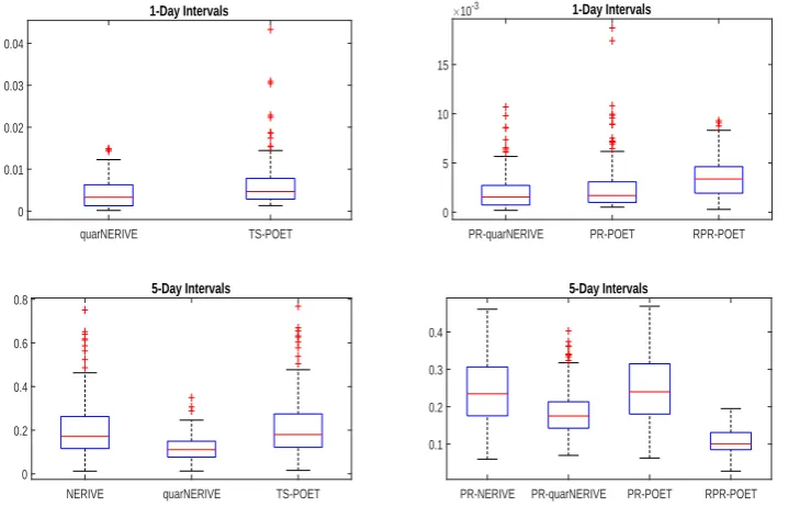
4.1 Mean and standard deviation of Frobenius error and average bias of eigenvalues over different 5-day or 1-day intervals for various methods. All values are multiplied by 10000. . . 105

4.2 Simulation results for model 1 with 5-day training window and no factors (C = 0 in (4.14)) . . . 111

4.3 Simulation results for model 1 with 1-day training window and no factors (C = 0 in (4.14)) . . . 112

(12)

List of tables xii

4.5 Simulation results for model 2 with 1-day training window and factors (C = 1 in (4.14)) . . . 114

4.6 Empirical results for the 26 most actively traded stocks in NYSE: 5-day training window . . . 115

4.10 Empirical results (jumps removed) for the 26 most actively traded stocks in NYSE: 5-day training window . . . 120

5.1 Mean losses for different methods, with standard errors in subscript. For the Frobenius loss, all values reported are multiplied by 10000. The realized covariance matrix is poorly conditioned when n =p= 200, so

the inverse Stein loss does not exist. . . 154

(13)

Chapter 1

Introduction

Estimation of a covariance matrix or its inverse, called the precision matrix, is an important and sometimes inevitable task in data analysis. Examples range from risk estimation and portfolio allocation in finance to classification or multiple hypotheses testing in general statistical analysis. Although it is easier than ever nowadays to obtain relatively large data set for study, such richness of data also means that more often than not the data we obtain are high-dimensional in nature, in the sense that the number of variables under study is comparable to or even larger than the sample size. This creates problems for traditional estimator such as the sample covariance matrix. Well documented inBai and Yin (1993) and subsequent random matrix theory researches (see Bai and Silverstein(2010), for example), a particularly serious problem is that the eigenvalues of the sample covariance matrix are more extreme than their population counterpart. Moreover, when the dimension p is larger than the sample

size n, the sample covariance matrix is not invertible, where regularization is needed.

This thesis contains three parts where covariance matrix estimation under different data frequency settings is applied: weighted average of a rotation-equivariant and a regularized covariance matrix estimator under low-frequency setting, a nonparametri-cally eigenvalue-regularized integrated covariance matrix estimator and a nonlinear shrinkage estimator of large integrated covariance matrix under high-frequency setting. The thesis is organised as follows.

In Chapter 2, state-of-the-art regularization methods developed for covariance matrix estimation are reviewed. One main branch of the estimations assumes a special structure of the population covariance matrixΣ0 or the corresponding precision matrix

(14)

2

(Bickel and Levina,2008a; Cai and Liu, 2011;Rothman et al., 2009), bandable type structure (Bickel and Levina,2008b;Cai and Yuan,2012;Cai et al.,2010), and a factor structure (Fan et al.,2008,2011,2013). Another branch concerns with regularizing, or “shrinking”, the eigenvalues of the sample covariance matrix under the high-dimensional setting p/n→ c >0. Research include the linear shrinkage (Ledoit and Wolf, 2004)

and nonlinear shrinkage (Abadir et al., 2014; Huang and Fryzlewicz, 2015;Lam, 2016;

Ledoit and Wolf, 2012,2013).

While both branch of researches provide good estimators under different scenarios, there are no methods that can “take advantage” of what each branch of estimators can offer. In Chapter 3, we introduce an integration covariance matrix estimator that is a linear combination of a rotation-equivariant and a regularized covariance matrix estimator that assumed a specific structure for Σ0, under the practical scenario where

one is not 100% certain of which regularization method to use. By minimizing the Frobenius loss, we derive explicit formulae for the weights which can be estimated consistently, or even almost surely, through a data splitting scheme which is similar to the one in Lam (2016). To generalize, we can put two regularized estimators into the linear combination, each assumes a specific structure forΣ0. Our estimated weights can

then be shown to go to the true weights, and if one regularized estimator is converging to Σ0 in the spectral norm, the corresponding weight then tends to 1 and others tend

to 0 asymptotically. Extensive simulations also reveal that our estimator can indeed gather the advantages from a regularized estimator and perform well, even when the regularized estimator itself does not. We also show that our estimator is asymptotically efficient when compared to an ideal estimator constructed with the knowledge of Σ0.

In Chapter 4, we propose a nonparametrically eigenvalue-regularized integrated covariance matrix estimator (NERIVE) which does not assume a specific structure for the underlying integrated covariance matrix in high-frequency data analysis. Under such setting, the extreme eigenvalues of a realized covariance matrix are biased when its dimension pis large relative to the sample size n. Together with non-synchronous

trading and contamination of microstructure noise, the associated challenges have to be overcome at the same time. By a data splitting method, we show that the resulting integrated covariance matrix estimator is consistent with a certain positive definite matrix with regularized eigenvalues at a rate ofn−1/6 under the settingp/n→c >0.We

(15)

3

the theoretical minimum variance portfolio weights. All these results hold true also under a jump-diffusion model for the log-price processes with jumps removed using the wavelet method proposed in Fan and Wang (2007). They are further extended to accommodate the existence of pervasive factors such as a market factor under the setting p/n→c >0. The practical performance of NERIVE is tested by a traditional

portfolio allocation problem, where our estimator is compared to other state-of-the-art estimators including the usual two-scale realized covariance matrix.

Finally in Chapter 5, we modify the data splitting method similar to NERIVE to achieve nonlinear shrinkage of eigenvalues in a covariance matrix. It produces a positive definite estimator of the integrated covariance matrix asymptotically almost surely, and involves only eigen-decompositions of matrices of size p×p, which are not

computationally expensive when p is of the order of hundreds, the typical order in

(16)

Chapter 2

Review on Covariance Matrix

Estimation

In this chapter, we provide a review on the estimation of covariance matrix or its inverse (known as precision matrix) related to this thesis, as well as the most popular state-of-the-art covariance estimators in applications for both high-dimensional and high-frequency data setting.

The most commonly used estimator is the sample covariance. LetY = (y1, . . . ,yn),

whereyt = (y1t, y2t, . . . , ypt)T’s are independentp×1 vectors for t= 1, . . . , n, being the

data observed at timet, for example, the stock market daily returns. LetΣ0 = (σij)p×p

be the population covariance matrix. The p×p sample covariance matrix is defined as

b

Σ_sam= 1

n−1

n

X

t=1

(y_t−y¯)(y_t−y¯)T

,

where ¯y= 1_nPn

t=1yi is the sample mean. Σb_sam is an unbiased estimator and easy to calculate. We can also use the maximum likelihood estimation (MLE) of the covariance matrix

b

ΣMLE =

1

n

X

t=1

(yt−y¯)(yt−y¯)T.

for the Gaussian distributed data. The use of the coefficient 1/n instead of 1/(n−1)

(17)

2.1 Estimation of Covariance Matrix through Thresholding 5

We enjoy the simplicity of the calculation ofΣb_samandΣb_MLE, however, they are well known to have poor performance when the dimension pis larger than or comparable

to the sample size n. In this high-dimensional setting, sample covariance matrix is

no longer a consistent estimator as the eigenvalues of Σb_sam are not converging to the true ones based on the random matrix theory (Chen et al., 2013; Johnstone, 2001;

Marčenko and Pastur, 1967). Also, its inverse, the sample precision matrix Σb−_sam1 , is not defined due to the singular sample covariance matrix.

As a result, regularization is needed in high-dimensional covariance matrix estima-tion. There are two main branches for estimating a large covariance matrix nowadays: one assumes a specific structure of the population covariance matrix, sparsity as an example; the other branch focuses on regularizing, or we say ’shrinking’, the eigenvalues of the sample covariance matrix. Here, we start from the sparsity setting of the large covariance estimation.

2.1

Estimation of Covariance Matrix through

Thresh-olding

2.1.1

Simple Thresholding

To deal with the ill-conditioned estimation problem of sample covariance matrix in high-dimensional setting, thresholding is one of the simplest method to apply under the assumption that the population covariance matrix is sparse or approximately sparse, i.e. most of the non-diagonal elements in the matrix are zero or nearly but not exactly zero (Bickel and Levina, 2008a). The uniformity class of the approximately sparse covariance matrices is defined as

U(q, c0(p), M) = {Σ:σii ≤M,max i

p

X

j=1

|σij|q ≤c0(p)}, (2.1)

for 0≤q <1. If q = 0, the matrix is truly sparse; otherwise 0< q <1, the matrix is

(18)

new estimator Σb_thre= ( e

σij)p×p defined as

e

σij =



 

  b

σij fori=j,

b

σij1{|_bσij|>ω} fori̸=j,

(2.2)

where1{·} is the indicator function andω is the threshold parameter. This is called the hard thresholding. They proved the consistency of this estimator if the variables yi’s are Gaussian or sub-Gaussian, uniformly on U(q, c0(p), M), logp/n = o(1), and

ω =C(logp/n)1/2 _{for sufficiently large} _C_,

∥Σb_thre−Σ₀∥=O_p(c₀(p)ω1−q), ∥Σb−_thre1 −Σ−₀1∥=O_p(c₀(p)ω1−q),

where ∥·∥ is the operator norm, also known as spectral norm or l2 matrix norm, as

∥A∥=λ1/2 max(A

T_A) for any matrix _A. The choice of threshold _ω can be estimated by

cross-validation method.

Thresholding decreases the estimation errors for small valued elements, since the errors are not accumulated with estimation. On the other hand, choosing elements that should be thresholded is always easier than estimating these small values. Although positive definiteness of Σb_thre cannot be gaurenteed, the probability of it being positive definite is approaching to 1 as long as logp/n → 0. Despite on the simplicity and

computational advantage, simple thresholding neglects the difference of covariance scales, i.e. the observed data series are usually on different scales. To solve the scale inconsistency problem, Cai and Liu (2011) proposed the entry-depandent adaptive thresholding, taking varying scales into account.

2.1.2

Adaptive Thresholding

One of the most natural and simplest solutions to deal with the variability of variances is to threshold on the sample correlation matrix instead of the sample covariance matrix. Denote the population correlation matrixR0 = (rij)p×p and sample correlation

matrix cR_sam = (r_b_ij)_p_×_p, where r_b_ij =σ_b_ij/ q

b

σiiσbjj. The thresholded correlation matrix estimator Rc_thre = (r_e_ij)_p_×_p is defined by

e

rij =



 

  b

rij fori=j,

b

rij1{|

brij|>ω} for

(19)

and the corresponding covariance matrix isΣb_R =D1/2cR_threD1/2, whereDis the diagnal matrix of the sample covariance matrix Σb_sam. It is easily to see that ω =C

q

logp/nis

a good threshold choice for any constant C >0, and if C is sufficiently large, it can be

shown that minimax rate of convergence is c0(p)ω1−q, same as the simple thresholding

above. This method well solves the variability of variance, nevertheless, the sample correlation coefficients rbij’s are still not homoscedastic.

As a result, the entry-depandent adaptive thresholding is introduced. Here, a new larger class of sparse covariance matrices (Cai and Liu, 2011) is defined by

Uadp(q, c0(p)) ={Σ: max

i p

X

j=1

(σiiσjj)(1−q)/2|σij|q ≤c0(p)}, (2.3)

for 0 ≤ q < 1. The parameter space Uadp₍_{q, c}

0(p)) contains the uniformity class

U(q, c0(p), M) defined in equation (2.1), and it allows the largest variance maxiσii → ∞,

not requiring the variances uniformly bounded by M any more. Different from the

simple thresholding, the threshold ω is not universal, but changing with the entries. It

is defined as

ωij =δ

s

b

θijlog

p

n , i, j = 1, . . . , p,

where

b

θij =

1

n

X

t=1

[(Yit−Y¯i)(Yjt−Y¯j)−σbij]

2_, _(2.4)

with ¯Yi being the sample mean of the ith row of the observed data matrix Y, and

b

σij being the corresponding sample covariance element. Note that the regularization

parameter δcan be chosen by cross-validation, or just be set fixed to 2 as recommonded

by Cai and Liu(2011). Then the adaptive estimator of covariance matrix is Σb_adp = (σb

adp

ij )p×p with

b

σadp_ij =



 

  b

σij fori=j,

b

σij1{|_bσij|>ωij} fori̸=j.

Alternatively,Σb_adp = ( b

σadp_ij )p×p can be defined in an universal entry independent way

as

b

σadp_ij =



 

  b

σij fori=j,

b

σij1_{|

bσij|/bθ

1/2

ij >ω} for

(20)

whereθb1/2

ij is the estimated standard error of the estimated covariance elementσbijdefined in equation (2.4), and ω is the universal threshold same as the simple thresholding

method (Bickel and Levina,2008a). It is shown that Σb_adp achieves the optimal rate of convergence c0(p)ω1−q over the parameter space Uadp(q, c0(p)).

2.1.3

Generalized Thresholding Function

Other than the hard thresholding used above, there are more complex thresholding functions that can be applied, for example, soft-thresholding. Rothman et al. (2009) proposed a generalized thresholding function sω : R → R, for any ω and z ∈ R,

satisfying the following three conditions:

1. |sω(z)| ≤ |z| ;

2. sω(z) = 0, for |z| ≤ω;

3. |sω(z)−z| ≤ω.

Condition 1 establishes the shrinkage. Although the bias increases, the variances are reduced and the estimator is more stable. Condition 2 enforces the thresholding, and Condition 3 limits the amount of shrinkage to no more than ω. Note that the

parameter ω in the last two conditions can be different. Most of the commonly used

thresholding procedures satisfy these conditions, such as the hard thresholding as we discussed above, and the soft thresholding proposed by Donoho and Johnstone (1994) which is defined as

ssoft_ω (z) =z1{|z|>ω}. (2.5) Moreover, the Smoothly Clipped Absolute Deviation (SCAD) penalty proposed by

Fan and Li (2001) (see Chapter 2.1.4) and Adaptive LASSO proposed by Zou (2006) are both special cases of the generalized thresholding function sω(z). It is shown that,

uniformly on the class U(q, c0(p), M), forω =C q

logp/n where C is sufficiently large,

∥sω(Σb)−Σ₀∥=O_p(c₀(p)ω1−q).

For the generalized thresholding, the corresponding covariance estimator is defined as

b

Σgen= (σb

gen

ij )p×p, σbij = 

 

  b

σij, fori=j,

sω(σbij), fori̸=j.

(21)

The disadvantage of thresholding is that the estimator is not positive definite for certain.

2.1.4

Penalized Likelihood

Penalized likelihood is another powerful method for exploring sparsity. Dempster(1972) recognised the inverse covariance matrix as the canonical parameter of a multivariate normal distribution, through whih the parsimony can be identified through modified Cholesky decomposition. The nonredundant entries of this matrix are the regression coefficients of one variable based on its predecessors, so that the task of modelling a covariance matrix can be reduced to that of modelling regression models (Wu and Pourahmadi, 2003), where penalized likelihood function can be used to shrink the off-diagonal elements of the matrix.

Antoniadis and Fan(2001) proposed a penalty function (2.6) with similar properties to the generalized thresholding function in Chapter2.1.3. Considering a linear regression model

y=Xβ+ϵ

where parameterβis ad×1 vector,yandϵaren×1 vectors and the design matrixXis an×dmatrix. βcan be estimated by solving the penalized least squares minimization

problem

1

2∥y−Xβ∥2+

d

X

j=1

pλ(|βj|),

wherepλ(·) is a penalty function with parameter λ. Naturally, ifL0 penalty is used,

pλ(|β|) =λ1{β̸=0}, it will lead to the Best-Subset selection. It finds the subset of sizek that gives the smallest residual sum of squares ∥y−Xβ∥2 for _k= 0_,1_{, . . . d}. The_L

1

penalty pλ(|β|) =λ|β| yields to the soft thresholding rule as stated in equation (2.5),

or Least Absolute Shrinkage and Selection Operator (LASSO) (Tibshirani,1996) in the general least squares and likelihood settings. Moreover, the L2 penalty pλ(|β|) =λ|β|2

gives a ridge regression and theLq penaltypλ(|β|) =λ|β|q results in a bridge regression.

And if we take pλ(|β|) =λ2−(|β| −λ)21{|β|<λ}, it will lead to the hard thresholding rule stated in equation (2.2).

The penalty functions we discussed above do not simultaneously satisfy the three properties for a good penalty function: unbiasedness, sparsity and continuity. Therefore,

(22)

2.2 Estimation of Covariance Matrix with Bandable Structure 10

defined by

p′_λ(β) =λ{1{β≤λ}+ (

aλ−β)+

(a−1)λ 1{β>λ}},

for some a >2 and positive β. Here (a)+ = max(0, a). The corresponding piecewise

linear thresholding function is then

sλ(z) =



    

    

sgn(z)(|z| −λ)+ for |z| ≤2λ,

[(a−1) −sgn(z)aλ]/(a−2) for 2λ≤ |z| ≤aλ, z for |z|> aλ.

SCAD can be seen as a combination of the soft and hard thresholding penalty functions, with improvements in the properties of these two penalty functions, selecting significant variables without creating excessive biases. The amount of shrinkage decreases when the magnitude of z rises. Note thata = 3.7 is suggested byFan and Li

(2001).

2.2

Estimation of Covariance Matrix with

Band-able Structure

Apart from assuming the sparse structure of the true covariance matrix, other popular assumptions on matrix sturcture are widely used as well, for example the bandable structure, where the elements of the matrix decay while moving away from the diagonal. Introduced by Bickel and Levina (2008b), we consider the following class of positive definite symmetric well-conditioned matrices

Uband₍_{α, M, C}_{) =}_{_Σ_{: max}

j

X

i

{|σij|:|i−j|> k} ≤Ck−α for all k > 0,

and 0<1/M ≤λmin(Σ)≤λmax(Σ)≤M <∞}, (2.7)

whereλmin(·) and λmax(·) represent the maximal and minimal eigenvalues of the matrix.

(23)

2.2.1

Banding

Bickel and Levina (2008b) proposed to estimate the covariance matrix by banding the sample covariance matrix Σb_sam as

b

Σband(k) = (σbij1{|i−j|≤k})p×p

for some 0 ≤ k < p. It can also be written as the Schur products of the sample

covariance matrix and a banding matrix Bk, defined as

Bk = (1{|i−j|<k})1≤i,j≤p.

The estimator Σb_band(k) = Σb_sam ◦B_k, where ◦ represents the Schur coordinate-wise matrix multiplication.

This regularization works ideally when the population covariance matrix element

σij = 0 for|i−j|> kafter arranging the indexesi’s of the observed datayit, t= 1, . . . , n

under some special way, for example finite inhomogenous moving average process

yit=Pkm=1at,t−mϵm with independent and identically distributed mean zero ϵm.

They proved that the estimator Σb_band(k) is consistent under the operator norm if n−1log_p _→0, uniformly over _Uband. The rate of convergence is (_n−1log_p)α/2(α+1)

with parameterk ≍(n/logp)1/2(α+1). Due to the lack of information on the decay rate

α in real case studies, K-folded cross-validation is recommended to better choose the

parameter k in banding method.

Banding method discards the off-diagonal entries of the sample covariance matrix that arek step away from the main diagonal, setting those values to zero, while keeping

the sub-diagonal or super-diagonal elements near the main diagonal unchanged. It can be generalized to the ’tapering’ method, where the elements gradually decay while moving away from the main diagonal of the matrix.

2.2.2

Tapering

(24)

The tapering estimator is defined as the Schur products of the sample covariance matrix and tapering matrix Tk = (wij)p×p as

b

Σtaper(k) =Σb_MLE◦T_k = ( b

σij ·wij)p×p,

for some even integer k with 1≤k ≤p, and the weights wij =



    

    

1 for |i−j| ≤k/2,

2−|i_k/−₂j| for k/2<|i−j|< k,

0 for |i−j| ≥k.

For simplicity, the weights can also be written as

wij = (k/2)−1{(k− |i−j|)+−(k/2− |i−j|)+}.

Over the parameter space Uband₍_{α, M, C}_{) defined in equation (}_2.7_{), this estimator} b

Σtaper(k) was proven to obtain the optimal rate of convergence n−2α/(2α+1)+ (logp)/n

under operator norm with parameter k ≍n1/(2α+1)_.

Compared with the rate of convergence of banding estimatorΣb_band(k), which was shown to be sub-optimal, Cai et al. (2010) proved the minimax rate of convergence for

b

Σtaper(k) is indeed optimal.

The estimatorΣb_taper(k) can also be written as the sum of many small block matrices along the main diagonal, and the size of the small blocks depends on the decay rate α.

2.2.3

Block Thresholding

As banding and tapering estimators are critically depending on the decay rateα, which

is unknown in practice, Cai and Yuan (2012) introduced an adaptive estimator Σb_block, independent of α and obtaining the optimal rate of convergence as we discussed in last

section.

Under the same class setting as equation (2.7), Σb_block is a data-driven block thresholding method constructed in two steps. First, the sample covariance matrix

b

Σsam is divided into small blocks with different size. By choosing the size k0 = ⌊logp⌋

(25)

2.3 Estimation of Covariance Matrix with Factor Analysis 13

the diagnal. The floor function ⌊a⌋represents the greatest integer less than or equal to

a. Then estimating the entries in each block by thresholding simutaneously such that:

• For the blocks located in the diagonal: keep their original values;

• For the large blocks whose dimension is larger thann/logn, ’kill’ them by setting

these blocks as 0;

• For other blocks, threshold them by a certain thresholding rule, for example, hard thresholding, soft thresholding or adaptive Lasso.

This entire data-driven estimatorΣb_block benefits from no requirement to chooseα, and Cai and Yuan (2012) showed that it simultaneously attains the optimal rate of convergence n−2α/(2α+1)_{+ (log}_p₎_/n _{for estimating bandable covariance matrices over}

the full range of the parameter spaces Uband(_{α, M, C}).

Block thresholding has a wide range of applications, such as financial stock market prices. Traditional thresholding, as we discussed in Chapter2.1, requires the assumption of sparsity, which the stock market along with a lot types of other empirical data cannot satisfy. In financial portfolio management, simple sparsity is not realistic for some cases, as the stock prices for similar type of stocks will have high correlation. As a result, the reasonable assumption in practice is to assume a block structure of the population covariance matrix, which is that the data are divided into groups or blocks by their features.

2.3

Estimation of Covariance Matrix with Factor

Analysis

(26)

introduced. The benefit of factor modelling comes from the reduction of dimensions, that the number of parameters needed for estimation is reduced significantly from

p×(p+ 1)/2 parameters to p×(K+ 1) for the best scenario, where K is the number

of factors and 0≤K < p.

Let yt = (y1t, . . . , ypt)T be the observed data at time t= 1, . . . , n, the factor model

is defined by

yt=at+Bft+ut, (2.8)

whereatis ap-dimension vector of data means,B = (b1, . . . ,bp)T is ap×K matrix of

factor loadings,ftis a vector of common factors in dimensionK, andut= (u1t, . . . , upt)T

is a vector of idiosyncratic components, i.e. error or noise terms.

2.3.1

Factor Model with Observable Factors

Factor models have been widely used both theoretically and empirically in economics and finance, such as the famous Fama and French three factor model, Capital Asset Pricing Model (CAPM), and Arbitrage Pricing Theory (APT). In some applications, the factors can be observed, such as the Fama and French three factor model, in which the excess return, market capitalization and book-to-market ratio are the three factors considered. Without loss of generality, we assume the mean vector at=0 in equation

(2.8), and the factors ft are independent of the noises ut. The factor model covariance

matrix estimator for yt is

ΣFM=BΣfBT+Σu, (2.9)

where Σf and Σu are the covariance matrices for factorsft and noises ut, respectively.

If we further assume the cross-sectional independence among the idiosyncratic components, which implies that the noise covariance matrix Σu = diag(σ1, . . . , σp) for

utis diagonal, we call this a strict factor model (Fan et al.,2008). Here, diag(a1, . . . , am)

denote the diagonal matrix of dimensionmwhose diagonal elements equal toa1, . . . , am

and off-diagonal elements are all zero. After regressing on yt, estimation of loading

matrix Bb and the residuals Σb_u = diag(σ_b₁, . . . ,σ_b_p) can be obtained. Bb = (bb₁, . . . ,bb_p)T can be estimated by applying the least squares estimation as

b

bi = arg min

bi

1

n

X

t=1

(27)

andubt= yt−Bfb t. Since the factorsft’s are observable,Σbf is just the sample covariance matrix for the factors. The resulting estimator for strict factor model is given by

b

ΣSFM =BbΣb_fBbT+Σb_u.

For any matrixA, the Frobenius norm is defined as ∥A∥F ={tr(AAT)}1/2. Under

the Frobenius norm, the dimensionality reduces the rate of convergence by the order of

pK, same as that of the sample covariance matrix. Since the sample covariance matrix

achieving the optimal rate as well, the factor structure does not give many advantages in estimating the population covariance matrix.

On the other hand, in the aspect of estimating the precision matrix Σ−₀1, it can be estimated by using the Sherman-Morrison-Woodbury formula as

b

Σ_SFM−1 =Σb−_u1−Σb−_u1Bb(Σb−1

f +Bb

T

b

Σ_u−1Bb)−1BbTΣb−_u1.

Fan et al.(2008) proved thatΣb−1

SFM performs much better thanΣb −1

sam when the number

of factor K =O(p).

Compared to the sample covariance matrix, Σb_SFM gets better convergence rate for estimating the precision matrix Σ−₀1 but the same rate for estimation of Σ0. As a

result, factor modelling performs better in portfolio allocation, but not much for risk assessment.

Strict factor model requires the chosen factors explaining all relationships between the data, which is too restricted to satisfy in practical sense. The approximate factor model estimator Σb_AFM is introduced by Fan et al. (2011), loosing the strict diagonal structrue of error covariance matrix to an approximate diagonal structrue. This allows the existence of small valued off-diagonal entries in estimated idiosyncratic matrix, suggesting the allowance of the presence of cross-sectional correlation even after taking out the common factors. The estimator is defined as

b

ΣAFM =BbΣb_fBbT+Σe_u.

(28)

thresholding (Cai and Liu,2011) is used to regularize Σb_u = ( b

σu,ij)p×p as

e

Σu = (σeu,ij)p×p, σeu,ij = 

 

  b

σu,ij i=j,

sω(σbu,ij) i̸=j,

wheresω(·) is the general thresholding function and here adaptive threshodingsω(σbu,ij) = b

σu,ij1{|_bσu,ij|>ωij} is applied in their paper (see Chapter 2.1.2 for adaptive thresholding

and Chapter 2.1.3 for generalized thresholding function).

Fan et al. (2011) proved that the estimated covariacne matrix is still invertible after thresholding even if p > n. It is clearly shown that p can be much larger than n when estimating the precision matrix. Eigenvalues ofΣb_AFM diverge quickly while those ofΣb−_AFM1 are uniformly bounded, suggesting a good performance of the estimated precision matrix also for approximate factor structure.

2.3.2

Factor Model with Unobservable Factors

In many practical applications, the common factors are always unobservable, i.e. latent. So estimation of the latent factors are needed. We apply the pervasive assumption that the number of factors K are bounded and eigenvalues of p−1BT_B are uniformly

bounded away from 0 and ∞ asp→ ∞.

We cannot observe the factors directly since they are latent. As the dimensionp

increases, the information about the common factors accumulates while that about the error terms does not. It helps to distinguish the factor term Bft from the idiosyncratic

term ut. As a result, the principal component analysis related method is widely used

in this field.

When the number of variables, i.e. dimension p, is large, we can use Principal

Component Analysis (PCA) to analyze the factor model. We assume that at =0 for

simplicity, and factor model in equation (2.8) is then

yt=Bft+ut = (BH)(H−1ft) +ut,

where H is a K ×K non-singular matrix. The solution for the pair (H,ft) is not

unique, caused by the problem of ’identifiability’ due to the unknown B and ft. To

solve the ambiguity of the solution, we further assume that the covariance of ft is a K

(29)

Similar to equation (2.9), the covariance matrix is defined as

ΣPC =BΣfBT+Σu =BBT+Σu,

where B = (b1,· · · ,bK). The K orthogonal columns bj, j = 1, . . . , K are in a

descending order according to the the norms ∥bj∥. For simplicity, we assume a strictly

descending order of ∥bj∥. It is easy to get the j-th eigenvector of B is the normalized

vectorbj/∥bj∥. The corresponding j-th largest eigenvalue is ∥bj∥2 for j < K, and 0

for the remaining p−K eigenvalues since

(BBT)

bj/∥bj∥= ( K

X

i=1

bjbTj)bj/∥bj∥=∥bj∥2bj/∥bj∥.

If the j-th factor satisfies the pervasive assumption, the eigenvalue ∥bj∥2 =Ppi=1b2ij is

of order p, and j-th factor influences a non-negligible fraction of the data Y among the p dimensions.

It is well known from linear algebra that the first K eigenvalues of BBT are the

same as those of BT_B. If _Σ

u =0 and ΣPC=BBT, the j-th eigenvlue ofΣPC =BBT

is

λj =



 

 

∥bj∥2 forj ≤K,

0 forj > K, (2.10)

and the corresponding eigenvector is

pj =bj/∥bj∥, (2.11)

making the covariance matrix be just the simple version of the spectral decompsition

ΣPC =

K

X

j=1

λjpjpTj.

If we allow a more general case ofΣu, the eigenvalues and eigenvectors in equations

(2.10) and (2.11) only hold approximately. By the Wely’s theorem and the sin(θ)

theorem of Davis and Kahan (1970), we have that

pj −bj/∥bj∥

= O(p

−1_∥_Σ

(30)

λj − ∥bj∥

2

≤ ∥Σu∥ for j ≤K, and |λj| ≤ ∥Σu∥for j > K. As a result, Σ0 ≈

K

X

j=1

λjpjpTj +Σu.

Under factor model assumptions, the firstK eigenvalues ofΣ₀ are very spiked, while the rest are either bounded or growing slowly. So the latent factors and the loadings can be approximated using the eigen-decomposition of Σ0. As a result, high-dimensional

factor model can be estimated by the principal component analysis.

To take advantage of the factor structure estimation and the sparseness exploitation in the error covariance matrix, Fan et al. (2013) proposed the Principal Orthogonal complEment Thresholding (POET) method for the approximate factor structure with sparsity, allowing the presence of some cross-sectional correlations.

POET uses the principal component analysis on the sample covariance matrix, and then thresholds the idiosyncratic matrix. Consider a factor model like equation (2.8) with at =0. The p×pcovariance matrix ofyt is given by Σ0 = BΣfBT+Σu. POET

assumes an approximate factor model that the first K eigenvalues of Σ0 are spiked

and grow at a rate O(p), andΣu is approximately sparse.

Now let λi and pi be the descending ordered eigenvalues and corresponding

eigen-vectors of the sample covariance matrix Σb_sam, and K be the number of diverging eigenvalues of Σ0. Then, the spectral decomposition of Σb_sam becomes

b Σsam=

K

X

i=1

λipipTi +Σbu,

whereΣb_u =Pp

i=K+1λbipbipb

T

i = (σbu,ij)p×p is the principal orthogonal complement. Due to the conditional sparsity assumption, they threshold on Σb_u as

e

Σu = (σeu,ij)p×p, σeu,ij = 

 

  b

σu,ii, i=j;

sω(σbu,ij), i̸=j,

wheresω(.) is a generalized thresholding function (see Chapter2.1.3), and the adaptive

thresholding sω(zij) =zij1{|_bzij|≥ωij} is suggested here. The POET estimator is then

b

ΣPOET =

K

X

i=1

(31)

2.4 Estimation of Covariance Matrix by Shrinkage 19

When K = 0, this estimator is the same as the simple adaptive thresholding (Cai and

Liu,2011) or more general thresholding cases depending on the choice of thresholding function (Rothman et al., 2009).

The estimator has an equivalent representation using a constrained least squares method with resultsBb = (bb₁, . . . ,bb_p) andbf_t. Let

b

uit =yit−bbT

ibft,σbu,ij =n −1Pn

t=1ubitubjt, and denote θb_ij = n−1Pn

t=1(ubitubjt−σbu,ij)

2_{. The adaptive threshold parameter for} _s

ω(·)

applied here is

ωij =C

q

b

θij ·(

1

√

p+

s logp

n ),

whereC > 0 is a sufficiently large constant.

Fan et al.(2013) proved that the estimated idiosyncratic matrix Σe_u and POET estimator Σb_POET are consistent estimators for Σ_u and Σ₀ respectively. With the increase of dimension p, more information can be provided. It is easier to distinguish

the factors with the noise, making this unknown factor case equivalent to the known factor one.

The advantage of this low rank with sparse matrix estimation is that POET is simple, optimization-free and it uses the data only through the sample covariance matrix.

For most empirical applications, the number of factorsK is unknown. The multi-fold

cross-validation method can be used to estimate K. After determining the estimated

parameter Kc, the POET method above then can be applied

b

ΣPOET = b

K

X

i=1

λippT+Σe_u.

2.4

Estimation of Covariance Matrix by Shrinkage

(32)

Researchers begin to find estimation methods that do not require assumptions on the structure of the true covariance matrix. Simple sample covariance matrix estimation does not assume any special structure, but the drawback is well-known that it is ill-conditioned when the dimension p is large relative to the sample size n.

Here, we introduce four cutting edge researches developing covariance estimation by shrinking the sample eigenvalues.

Stein(1956) first used this idea to estimate the mean vector. This shrinkage method is substituting the original ill-conditioned estimator with a convex combination of itself and a target matrix. It balances between the estimation error coming from the ill-conditioned variance matrix and the specification error associated with the target matrix.

2.4.1

Linear Shrinkage

There is one type of covariance matrix estimation combining linearly two or even more existing estimators. For example, Ledoit and Wolf (2004) proposed a well-conditioned estimator Σb_lin, which is the asymptotically optimal convex linear combination of the sample covariance matrix with the identity matrix under quadratic loss function.

Here, we define the condition number as the ratio of the maximal and minimal singular values of the estimator. If the condition number is not much larger than one, we say the matrix is well-conditioned, which means its inverse can be computed with good accuracy. If the condition number is very large, the matrix is said to be ill-conditioned. Practically, such a matrix is almost singular, and the computation of its inverse or the solution of a linear system of equations is more likely to cause large numerical errors. A non-invertible matrix has condition number equal to infinity. As a result, well-condition is a very important property that a good estimator should obtain.

Sample covariance matrix works well only if p ≪ n. For the estimation of large

covariance matrices, p is large and it is difficult to find enough samples with size n to

makep/n negligible. Whilep/n <1 but not negligible, the estimator may be invertible,

(33)

well-conditioned, a direct method is to force it to be well-conditioned in structure by diagonality or factor model for example. But the absence of prior information would lead the structure to be mis-specified in general.

To shrink sample covariance towards to the identity matrix,Ledoit and Wolf(2004) introduced a linear combination of sample covariance matrix and the identity matrix as,

b

Σlin =w·tr(Σb)/p·I_p+ (1−w)·Σb_sam, where

w= min1,

1

n2

Pn

i=1∥yiyTi −Σb∥2F

∥Σb −tr(Σb)/p∥2_F

.

Here, Ip is the identity matrix with dimension p, and w is the shrinkage intensity

measuring the amount of shrinkage ofΣb_samtowardsI_p. This weighted average of sample covariance and identity matrix is equivalent to linearly shrink the sample eigenvalues to the grand mean while retaining the sample eigenvectors.

In the general asymptotics framework, wherep/n→c > 0, the optimal shrinkage

intensity w can be estimated consistently. This estimator Σb_lin benefits from its free of distribution and computational advantage. Simulation results show that Σb_lin outperforms the sample covariance matrix and does well in finite sample version. More importantly, Σb_lin is better-conditioned, and always be invertible even when p > n.

2.4.2

Nonlinear Shrinkage on Eigenvalues

Different from their previous paper we discussed in last section applying the one-size-fits-all approach (Ledoit and Wolf, 2004), Ledoit and Wolf (2012) proposed a new rotation equivariant estimator focusing on the individualized shrinkage intensity to every sample eigenvalue. A covariance matrix estimator is rotation equivariant if and only if it has the same eigenvectors as the sample covariance matrix. As such an estimator, it can only differentiate itself by its eigenvalues.

To do this, the eigen-decomposition is applied in the sample covariance matrix by

b

(34)

whereP= (p1, . . . ,pp) and D= diag(λ1, . . . , λp) are thep×p matrix of eigenvectors

and p-dimension digonal matrix of all eigenvalues of Σb_sam, respectively.

Under large-dimensional asymptotics p/n→c∈(0,1) asn→ ∞, define Hn as the

empirical distribution function of the population covariance matrix and Fn as that

of the sample covariance matrix. Assume Hn converges to some limit H. Using the

Stieltjes transformation mFn(z),∀z ∈ C

+_{, the Marcenko-Pastur equation} _m

F(z) of

functionFn and the estimation offmF(λ)≡limz→λmF(z), they proposed the estimator through the minimization problem under Frobenius loss

min

A

PAPT₋

Σ0

_F

,

whereA= diag(a1, . . . , ap) is thep-dimension diagonal matrix. Ledoit and Péché(2011)

showed the solution for the minimization problem ai, i= 1, . . . , p can be approximated

by

e

ai =

λi

|1−c−cλifmF(λi)| 2,

where eai only depends on the limiting distribution of sample eigenvalues. Hence, they proposed an estimator Σb_nonlin through nonlinearly shrinkage of the sample eigenvalues:

b

Σnonlin=P·diag

e

ai

i=1,...,p·P

T

.

Simulation study shows a significant improvement over the sample covariance matrix

b

Σsam and the linear shrinkage estimator Σb_lin (Ledoit and Wolf,2004) when the sample size n is very large compared to the dimension p.

2.4.3

Condition Number Regularized Estimator

Based on the fact that orthogonal matrices are never ill-conditioned,Abadir et al.(2014) proposed a new rotation equivariant estimator by applying orthogonal decomposition of the sample covariance matrix under high-dimensional setting p/n→0.

The condition number of any orthogonal matrix is always equal to 1, so the ill-condition of the sample covariance matrix only comes from the eigenvalues part of

b

(35)

λi, i= 1, . . . , p. The estimated diagonal matrix of eigenvalues is

D =PT

b

ΣsamP= diag(var(pT1Y), . . . ,var(p

T

pY)). (2.12)

Now, instead of using the whole dataset Yto estimateP, onlym (m < n) observations

are used to approximately orthogonalize the rest of the n−m observations, which are

used to re-estimate D. Assumem → ∞and n−m→ ∞ as n→ ∞, and yi’s are i.i.d.

distributed. The reason of spliting the whole sample set is that D cannot reuse the data that has already been used for calculating P, since they worsen the estimate of D. Denote the whole data asY = (Y1,Y2), where Y1 has dimension p×m and Y2

has dimension p×(n−m). Here, Σe₁ and Σe₂ are the sample covariance of Y₁ andY₂, respectively. Define Σe₁ = P₁D₁PT₁, whereP₁ is the matrix of eigenvectors ofY₁. The new estimator for eigenvalues is then defined as

c

D= diag(var(PT

1Y2)) = diag(PT1Σe₂P₁),

and the resulting Condition number Regularized Covariance matrix estimator (CRC) is then defined as

b

ΣCRC =Pdiag(PT1Σe₂P₁)PT. (2.13)

Abadir et al.(2014) further improved the estimator by repeatly choose different sub-samples (Y1 and Y2) and taking the average of the estimators by all cases. For

simulation study, the split point is selected by balancing the trade-off between variance and bias through bootstraps.

Such an estimator reduces the multi-variate problem to punivariate ones, enabling

also the easy-to-apply estimation of the functions on Σ0, such as the estimation of

the precision matrix. Σb_CRC is also always design-free and well-conditioned even when

p > n.

2.4.4

NERCOME

Inspired by Abadir et al. (2014), Lam (2016) proposed a covariance matrix estimator that nonparametrically regularize the eigenvalues (NERCOME).

They first proved the theoretical properties of the regularized eigenvalues inAbadir et al. (2014). When the observations can be written as yi = Σ

1/2

0 zi, where zi’s are

(36)

are asymptotically the same as the nonlinearly shrunk ones in Σb_nonlin (Ledoit and

Wolf, 2012). The computer advantage for Σb_CRC cones from the only involvement of eigen-decompositions of p×pmatrices, while Σb_nonlin requiring nonconvex optimizations could be computational expansive.

Lam(2016) also showed that the nonlinear shrinkage formula in Ledoit and Wolf

(2012) is not correct if the data is from factor model, due to the low dimensional factors. The data splitting regularized eigenvalues are still asymtotically optimal when we consider the Frobenius loss minimization.

Relaxing from the high-dimensional settingAbadir et al. (2014) that p/n→0,Lam

(2016) considered p/n→c >0. They focused on the optimization problem

min

D ∥P1DP T

1 −Σ0∥F,

and the optimal solution for D = diag(d1, . . . , dp) is

di =pT1iΣ0p1i.

Through splitting the data into two independent parts, the estimated eigenvalues are the diagonal elements of matrix PT

1Σe₂P₁, same as those in Abadir et al. (2014). The estimator is similar toΣb_CRC in equation (2.13), expect thatPis substituted byP₁, the matrix of eigenvectors for the first m of the whole data,Y1, only. They proposed

the estimator as

b

Σm =P1diag(PT1Σe2P1)PT1.

The change from P to P1 makes sense due to their optimization problem under

Frobenius loss and they showed that the pT

1iΣe₂p₁_i is asytotically the same as d_i. Apparently, this estimator is not as informative asΣb_CRC, due to the change ofP₁. As a result, they announced the final estimator as the averaging over all Σb_m’s calculated by different choices of Y1 and Y2. Referring to the assumption that each vector yi inY

is independent of each other and identically distributed, the data Y can be permuted so that there can be multiple choices of data matrix Y₁(j) andY(₂j). The corresponding covariance estimator for jth _{permutation is} _Σ_b(j)

m and the final NERCOME estimator is

b

ΣNERCOME = 1

M

X

(37)

2.5 Estimation of Covariance Matrix in High Frequency Setting 25

They showed theoretically and empirically better performance of Σb_NERCOME, com-pared to Σb_CRC. The regularization of eigenvalues gives NERCOME asymptotically optimal nonlinear shrinkage with respect to Frobenius norm. Σb_NERCOME is positive defi-nite almost surely as long as the population covarianceΣ0is, even in a high-dimensional

setting (p > n).

2.4.5

NOVELIST

The linear combination of two covriance estimators can be considered as an other kind of nonlinear eigenvalue shrinkage. Huang and Fryzlewicz (2015) proposed a NOVEL Integration of the Sample and Thresholded covariance estimators (NOVELIST), performing shrinkage of the sample covariance / correlation towards its thresholded version.

DenoteRc_sam as the sample correlation matrix, and s_λ(·) as the generalized thresh-olding function (Rothman et al., 2009) with threshold λ (see Chapter 2.1.3). The

correlation version of NOVELIST is defined as

c

RNOVELIST = (1−δ)·cR_sam+δ·s_λ(cR_sam),

where δ is the weight parameter for the thresholded estimator. The corresponding

covariance version of NOVELIST is defined as Σb_NOVELIST= D1/2cR_NOVELISTD1/2, with D as the diagnal matrix the sample covariance matrix Σb_sam.

The parameters (λ, δ) do not have a theoretical optimal solution, so that they are

obtained by cross-validation or just a fixed set of parameter choice based on different scenarios in data analysis. Thanks to the flexible control of the degree of shrinkage and thresholding, NOVELIST, as a simple, good all-round covariance, correlation and precision matrix estimator, offer competitive performance across other covariance matrix estimation methods.

2.5

Estimation of Covariance Matrix in High

Fre-quency Setting

(38)

For example, in stock market, there are thousands of transactions for a stock every day, not even include the tons of bid and ask data. Why would investors only use the daily closing price, the low frequency data, for analysis? The dramatical increase in data will benefit the research through bringing lots of extra information, but it will also cause some problems. In this section, the problems caused by high-frequency data and possible solutions are discussed.

2.5.1

Integrated Variance

First, we only consider the simplest case, where the dimension equals to one. When the input data’s frequency increases, the common variance is no longer useful, as we are more interested in the total variation over a certain period, i.e. the integrated variance. The most commonly used estimator is the Realized Variance (RV). Let Xt

be the price process for stock return in logarithm, following an Ito process,

dXt=µtdt+σtdWt, t ∈[0,1],

where µt and σt are the drift and volatility terms which can follow some random

processes, and Bt is a standard Brownian motion. Under the continuous setting, the

quadratic variation, i.e. the true variance of our interest, is given by

[X] =

Z 1

0

σ_t2dt.

To estimate this variance, the commonly used method is called the realized variance or the quadratic covariation, defined as

[X] = lim

n→∞

n

X

i=1

(Xti −Xti−1)

2

, (2.14)

for any sequence of partitions 0 =t0 < t1 <· · ·< tn= 1 with supi(ti−ti−1)→0 for

n → ∞. Here Xti represents the i

th _{transaction price during the periond [0}_,_{1], and} _t

i

is the time when this ith transaction happens.

(39)

microstructure noise. Let Yti be the log-price we observe at time ti, it is equal to the

sum of true underlying log-price Xti and the microstru

Eigenvalue regularized covariance matrix estimators for high dimensional data