Upper and lower bounds for a reactive diffuse system with Arrhenius kinetics

SYSTEM WITH ARRHENIUS KINETICS

Received 7 December 2005; Revised 31 May 2006; Accepted 5 June 2006

Comparison arguments are used to study a problem in combustion theory consisting of a nonlinear parabolic equation together with initial and boundary conditions. Upper and lower bounds for the problem are constructed. The lower solutions are used to determine whether the solution of the problem is increasing in time for certain initial condition. Nu-merical results are presented for the slab, infinite cylinder, and unit sphere. The bounds are compared with the existing ones in the literature for the slab geometry.

Copyright © 2006 Hindawi Publishing Corporation. All rights reserved. 1. Introduction

In this paper we consider the nonlinear parabolic equation, which describes the reactive-diffusive problem for a nonisothermal permeable catalyst pellet with first-order Arrhe-nius kinetics. The governing equation in the nondimensional form is

∂θ

∂t = ∇2θ+λ2(β−θ)eδ(θ/(1+θ)), x∈Ω,t >0, (1.1) subject to homogeneous boundary condition of Dirichlet type and initial condition

θ(x, 0)=r(x)≥0. (1.2)

HereΩis a bounded domain ofRN_{and∂Ωis the smooth enough boundary ofΩ.θ(x,t) is} the temperature of the reacting species, andβ,δ, andλare nonnegative parameters which represent the chemical heat release, the activation energy of the reaction, and the Thiele modulus, respectively. All variables are considered nondimensionalized. The full deriva-tion of the system and extensive literature for early work can be found in [3]. The steady-state problem has been studied by many authors for the Dirichlet and Robin boundary conditions, see [5–9], and here is a summary of previous work. Kapila and Matkowsky [7] considered the problem on the slab and infinite cylinder and derived asymptotic ex-pansion for the solution with largeδ. They found that the behavior of the solution is

Hindawi Publishing Corporation

International Journal of Mathematics and Mathematical Sciences Volume 2006, Article ID 24391, Pages1–13

similar for both geometries and therefore only presented the results for the infinite cylin-der. For the slab geometry the steady-state system has been reduced to a single equation by integrating the governing differential equation twice, see [5]. The literature shows that for certain values ofδandβthere existλoandλo such that the steady-state system has multiple solutions forλo≤λ≤λo. Hereλoandλocorrespond to extinction and ignition limits, respectively, and the corresponding steady-state solutions are known as the middle solutions, whereas forλ > λoandλ < λothe unique steady-state solutions are known as the upper and lower solutions, respectively. The number of middle solutions depends on the geometry of the domainΩand the boundary conditions [6–8]. Of interest are the values ofλoandλo. An attempt to evaluate these values was made in [7] for the slab and infinite cylinder geometries using asymptotic expansion approach. Recently, Al-Refai [1] has considered the problem with Dirichlet boundary conditions. He proved the existence of a nonnegative solution and derived sharp upper and lower bounds for the values ofλ andδusing comparison theory. Also in [2] he derived analytical upperand lower bounds for the extinction and ignition limits for the three geometries: slab, infinite cylinder, and unit sphere. Although the steady-state problem may have more than one solution, the problem with time-dependent has a unique solution provided that 0≤θ(x, 0)≤β(see [10, page 42]).

In this paper, we study the time-dependent problem in the slab [0, 1], in the unit sphere, and infinite cylinder. InSection 2, we write some preliminary results for the sys-tem which will be used through the text. In Section 3, we construct upper and lower solutions for the problem (1.1)-(1.2). InSection 4, we present some numerical results in the three geometries. Finally, we write some concluding remarks inSection 5.

2. A preliminary result

We have the problem

Pθ=∂θ_∂t − ∇2_θ−λ2_{g(θ)=0, x∈Ω,t >0,} θ(x,t)=0, x∈∂Ω,

θ(x, 0)=r(x)≥0,

(2.1)

whereg(θ)=(β−θ)eδ(θ/(1+θ))_{. A well known result for the system is that 0≤θ(x,t)≤β} provided thatr(x)≤β. Ifδβ≤1, then

g_{(θ)= −}eδ(θ/(θ+1)) (θ+ 1)2

θ2_{+ (2 +δ)θ+ 1−δβ<0, (2.2)}

Proposition 2.1. Consider the problem in (2.1) withg(θ) being bounded. (i) If (∂θ/∂t)(x, 0)<0, then (∂θ/∂t)(x,t)<0 for all x∈Ω, andt≥0. (ii) If (∂θ/∂t)(x, 0)>0, then (∂θ/∂t)(x,t)>0 for all x∈Ω, andt≥0. For the proof one can see [4,12].

3. Upper and lower bounds

To construct upper and lower bounds for the problem we use maximum principle for parabolic equations, see [11, page 187]. Letw(x,t) andu(x,t) satisfy

Pw≤0≤Pu, x∈Ω,t >0, w(x,t)≤0≤u(x,t), x∈∂Ω,

w(x, 0)≤r(x)≤u(x, 0).

(3.1)

Thenw(x,t) andu(x,t) are lower and upper solutions for the problem in (2.1), respec-tively,w(x,t)≤θ(x,t)≤u(x,t), as long as both exist.

Letλ1 be the first eigenvalue andφ1 the corresponding normalized, with respect to L2_{-norm, eigenfunction of}

∇2_{φ= −λφ, x∈Ω,}

φ=0, x∈∂Ω. (3.2)

It is easily obtained thatφ1=√2 sin(πx), (1/√2π)(sin(πx)/x), andJ0(γ0x), for the slab, spherical, and cylindrical geometries, respectively. HereJ0(γ0x) is the Bessel function of order zero,γ0=2.404825...is the first zero ofJ0(x), and 0≤x≤1. In all cases, the first eigenfunctionφ1is nonnegative inΩ.

3.1. Bounds wheng(θ) is decreasing. We derive upper and lower solutions for the prob-lem whenδβ≤1 and sog(θ) is decreasing. The functiong(θ) has only one inflection pointθ0_{=(δβ−2β−2)/(δ+ 2 + 2β), andg(θ) is concave up forθ < θ}0_{and concave down} forθ > θ0_{. Forδβ≤1, we haveθ}0_{<0, and therefore,g(θ) is concave down on [0,β].}

Theorem 3.1. Letφ1andλ1be as defined in (3.2) and letφ1mbe the maximum ofφ1onΩ. Letk(t) be the solution of the IVP

k_(t)=λ2_{gk(t)−λ1k(t),}

k(0)=k0. (3.3)

Thenk0≤k(t)≤kmandw(x,t)=k(t)(φ1(x)/φ1m) is a lower solution of (2.1). Herekmis the unique solution ofg(km)=(λ1/λ2)kmandk0=k(0) is chosen such thatk0(φ1(x)/φ1m)≤ r(x).

Proof. Sinceg(0)=β >0, we have (λ1/λ2_{)u≤g(u) for 0≤u≤k}

and therefore,k0≤k(t)≤km. The analogous result is obtained ifkm≤k0≤β, butk(t) is decreasing. Now,

Pw=k φ1 φ1m+λ1k

φ1 φ1m−λ

2_g

k_φ1φ1 m

=_φ1φ1

mλ

2_g(k)−λ2_gk φ1 φ1m

≤λ2_g(k)−gk φ1 φ1m .

(3.4)

Since k(t)(φ1/φ1m)≤k(t) and g is decreasing, we have Pw≤0, which together with w(x, 0)≤r(x) proves thatwis a lower solution of (2.1).

Theorem 3.2. Letψbe the solution of

∇2_{ψ= −1, x∈Ω,}

ψ=0, x∈∂Ω. (3.5)

Thenψ≥0, andu(x,t)=h(t)ψ(x) is an upper solution of (2.1), where

h(t)=h0−_λ2g1

(0)

1−eλ2_g(0)t

, (3.6)

andh0=h(0) is chosen such thath0≥λ2_{βandh0ψ(x)≥r(x).}

Proof. To show thatψ≥0, letξ= −ψ, thenξ satisfies∇2_{ξ=1≥0, andξ=0 on∂Ω.} Using maximum principle of elliptic equations (see [11, page 64]), we haveξ≤0, and henceψ≥0. Sinceg(0)=δβ−1≤0, it is not difficult to see thath(t) is increasing with

h0≤h(t)≤h0+_λ2 1

(1−δβ), (3.7)

and it is the unique solution of the IVP

h_−λ2_g(0)h=0,

h(0)=h0>0, h(0)=1. (3.8)

Now,Pu=h_ψ+h−λ2_{g(hψ) and} ∂Pu

∂t =hψ+h−λ2hψg(hψ)=

h_−λ2_{hg(hψ)ψ+h. (3.9)}

Sinceh(t)ψ≥0 andgis decreasing, we have ∂Pu

∂t ≥

h_−λ2_{hg(0)ψ+h(t)=h(t). (3.10)}

Integrate the above inequality from 0 totto get

or

Pu≥ψ+h(t)−λ2_{gh0ψ≥h(t)−λ}2_{β≥0, (3.12)}

which together withu(x, 0)=h0ψ(x)≥r(x)≥0 proves thatuis an upper solution of

(2.1).

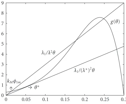
3.2. Lower solutions for δ >4 + 4/β. When δ >4 + 4/β, the inflection point θ0₌ (β(δ−2)−2)/(δ+ 2 + 2β)∈[0,β]. Letθ∗_{∈[0,β] be the smallest solution of (λ1/λ}2_)θ= g(θ) andλ1/λ2_{=g(θ), and letλ}∗_{be the corresponding value ofλ, seeFigure 3.1. For the} exact values ofθ∗andλ∗, one is referred to [2]. We have the following.

Proposition 3.3. (1)θ0_{=(β(δ−2)−2)/(δ+2β+2)> θ}∗_{=(β(δ−2)−βδ(βδ−4β−4))/} 2(β+δ) forδ >4 + 4/β.

(2) The functionh(θ)=g(θ)−(λ1/λ2_{)θis decreasing in [0,θ}∗_{] forλ≤λ}∗_.

Proof. (1) It is enough to show that

β(δ−2)−2 δ+ 2 + 2β >

β(δ−2)

2(β+δ), (3.13)

or

2(β+δ)β(δ−2)−2> β(δ−2)(δ+ 2β+ 2). (3.14)

The last inequality is equivalent to

βδ2_{−δ(4β+ 4)≥0. (3.15)}

Now, 4β+ 4< βδand hence−δ(4β+ 4)>−βδ2_{, which proves (3.15).}

(2) Sinceθ∗< θ0_{, we haveg(θ) increasing in [0,θ}∗_{] and henceh(θ)=g(θ)−λ1/λ}2_≤ g_(θ∗_)−λ1/(λ∗₎2_{=0, which proves the result.}

Theorem 3.4. Letφ1andλ1be as defined in (3.2) and letφ1mbe the maximum ofφ1onΩ. Forλ≤λ∗_{, letk(t) be the solution of the IVP}

k_(t)= 1 φ1m

λ2_gk(t)φ1

m−λ1k(t)φ1m,

k(0)=k0, (3.16)

wherek0≤kM is chosen such thatk0φ1(x)≤r(x), andkM is the solution (the smallest so-lution if there is more than one) ofλ2_g(k

0 0.05 0.1 0.15 0.2 0.25 0.3

θ

0 1 2 3 4 5 6 7 8 9

kMφ1m

λ1/λ2θ

g(θ)

λ1/(λ

)2θ

Figure 3.1. The values ofθ∗_{andkM, forβ=0.3 andδ=25.}

Proof. Sincek0≤kMand (λ1/λ2)φ1mu≤g(φ1mu) for 0≤u≤kM, we havek(t) increasing with equilibrium valuekM, that is,k0≤k(t)≤kM. Now,

Pw=k_{(t)φ1+λ1k(t)φ1−λ}2_gk(t)φ1

=_φ1φ1

m

λ2_gkφ1

m−λ1kφ1m+λ1kφ1−λ2gkφ1

≤λ2_gkφ1

m−λ1kφ1m−λ2gkφ1−λ1kφ1.

(3.17)

Sinceg(θ)−(λ1/λ2_{)θis decreasing in [0,θ}∗_{] forλ≤λ}∗_{, we havePw≤0 and the result}

is obtained.

Theorem 3.5. Forλ > λ∗, let(λ)>1 be such thatg(θ∗)=(λ1/λ2_)θ∗_{, and letk(t) be the}

solution of

k_(t)= 1 φ1m

λ2_gk(t)φ1

m−λ1k(t)φ1m,

k(0)=k0, (3.18)

wherek0≤θ∗_{/φ1m is chosen such that k0φ1(x)≤r(x). Then the functionh(θ)=g(θ)−} (λ1/λ2_{)θis decreasing in [0,θ}∗_{] andw(x,t)=k(t)φ1(x) is a lower solution of (2.1).}

in [0,θ∗_{] and>1 we have}

Pw=k_{(t)φ1+λ1k(t)φ1−λ}2_gk(t)φ1

=_φ1φ1

m

λ2_gkφ1

m−λ1kφ1m−λ2gkφ1−λ1kφ1

≤λ2_gkφ1

m−λ1kφ1m−λ2gkφ1−λ1kφ1

=λ2

gkφ1m−λ1_λ2kφ1m −

gkφ1−λ1_λ2kφ1 ≤0,

(3.19)

which proves the result.

4. Numerical results

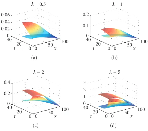
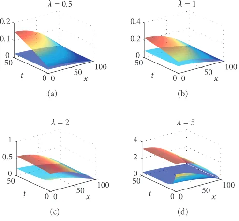
We consider the case where g(θ) is decreasing, and use Theorems 3.1 and 3.2 to ob-tain lower and upper solutions of (2.1). We present the bounds for different values of λ,β,δ and 0≤t≤0.2, with initial conditionθ(x, 0)=λ2_{βψ(x), whereψ(x) is defined} in Theorem 3.2. Figures4.1,4.2, and4.3depict these bounds of the problem whenΩ is the slab, unit sphere, and infinite cylinder, respectively, andβ=0.5,δ=0.1, andλ=

0.5, 1, 2, 5. In order for the conditionk0(φ1/φ1m)≤r(x) to be satisfied inTheorem 3.1, we takek0=λ2_β/8,λ2_β/18.9,λ2_{β/6.4, for the slab, sphere, and infinite cylinder, respectively.} From the figures one can see that the upper bounds are increasing in time, where

h(t)=λ2_β+ 1 λ2

1 1−δβ

1−e−λ2_(1−δβ)t

, (4.1)

whereas the lower bounds are decreasing or increasing in time, depending on the geome-tryk0andkm. For example, the lower solutions are decreasing in time in the slab geometry sincek0> km, while they are increasing with time forλ=0.5, 1, 2 and decreasing forλ=5 in the sphere.Table 4.1showsk0 andkm, forβ=0.5,δ=0.1, and different values ofλ. Also, the upper and lower solutions are close to each other and give good information about the exact solutionθ.

FromProposition 2.1we have that ifθt(x, 0) =0, then the solutionθis either increas-ing or decreasincreas-ing in time. We now takeθ(x, 0)=cφ1(x) and ask the following: for what values ofcthe solutionθof (2.1) is increasing with respect to time? To answer the ques-tion, we substitutek0=cφ1m in Theorem 3.1. Sinceθ(x, 0)=w(x, 0) andw(x,t) is in-creasing in time forc < km/φ1m, then so isθ.

Finally, we compare our bounds with the bounds obtained in [10]. Consider the PDE ∂v

∂t = ∇2v−λ2c0v+μ0β, x∈Ω, v(x,t)=0, x∈∂Ω,

v(x, 0)=r(x)≥0,

(4.2)

100 ₅₀ 0

x 40 20

0

t

0 0.01 0.02 0.03 0.04 0.05

λ=0.5

(a)

100 50

0

x ₄₀ 20

0

t

0 0.05 0.1

λ=1

(b)

100 50

0

x 30 20t10 0

0 0.1 0.2 0.3 0.4

λ=2

(c)

100 ₅₀ 0

x 40 20

0

t

0 0.5 1 1.5 2

λ=5

(d)

Figure 4.1. Upper and lower bounds for the slab geometry, whenβ=0.5,δ=0.1, andλ=0.5, 1, 2, 5.

40 20

0

t 0 50

100

x

0 0.02 0.04 0.06

λ=0.5

(a)

40 20

0

t 0 50

100

x

0 0.1 0.2

λ=1

(b)

40 20

0

t 0 50

100

x

0 0.2 0.4

λ=2

(c)

40 20

0

t 0 50

100 x 0 1 2 3

λ=5

(d)

Figure 4.2. Upper and lower bounds for the spherical geometry, whenβ=0.5,δ=0.1, andλ=

50

0

t ₀ 50 100

x

0 0.1 0.2

λ=0.5

(a)

50

0

t ₀ 50 100

x

0 0.2 0.4

λ=1

(b)

50

0

t ₀ 50 100

x

0 0.5 1

λ=2

(c)

50

0

t ₀ 50 100

x

0 2 4

λ=5

(d)

Figure 4.3. Upper and lower bounds for the cylindrical geometry, whenβ=0.5,δ=0.1, andλ=

0.5, 1, 2, 5.

Table 4.1. The values ofk0andkm, forβ=0.5 andδ=0.1, in the three geometries.

λ 0.5 1.0 2.0 5.0

Slab k0 0.015625 0.062500 0.250000 1.562500

km 0.012367 0.046185 0.145507 0.361155

Sphere k0 0.006614 0.026455 0.105820 0.661380

km 0.012367 0.046185 0.145507 0.361155

Cylinder k0 0.019531 0.078125 0.312500 1.953100

km 0.020759 0.074147 0.206504 0.408257

geometry we have

v(x,t)=2β_π ∞

n=1

1−(−1)n n

_λ2 n2π2e

−rnt₊μ0

rn

1−e−rntsin(nπx),

v(x,t)=2βλ_π2 ∞

n=1

1−(−1)n n

1 n2π2e

−rnt₊ 1

rn

1−e−rntsin(nπx),

(4.3)

wherern=n2π2+λ2μ0andμ0=1.033895.

0 10

20

x 40 20

0

t

0 0.02 0.04 0.06

λ=0.1

(a)

0 10 20

x 40 20t 0

0.01 0 0.01 0.02 0.03 0.04

λ=0.1

(b)

0 10

20

x 40 20

0

t

0 0.02 0.04 0.06

λ=0.5

(c)

0 10

20

x 30 20_t10 0 0.01

0 0.01 0.02

λ=0.5

(d)

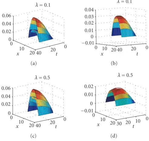
Figure 4.4. The upper solutionsu(x,t) andv(x,t) and the differencev(x,t)−u(x,t) for the slab ge-ometry, whenβ=0.5,δ=0.1, andλ=0.1, 0.5.

0 20

40

t ₀ 10 20

x

0 0.05 0.1

λ=1

(a)

0 _{20 40}

t 0 10

20

x

0.04 0.02 0 0.02

λ=1

(b)

0 20

40

t ₀ 10 20

x

0 0.5 1 1.5

λ=4

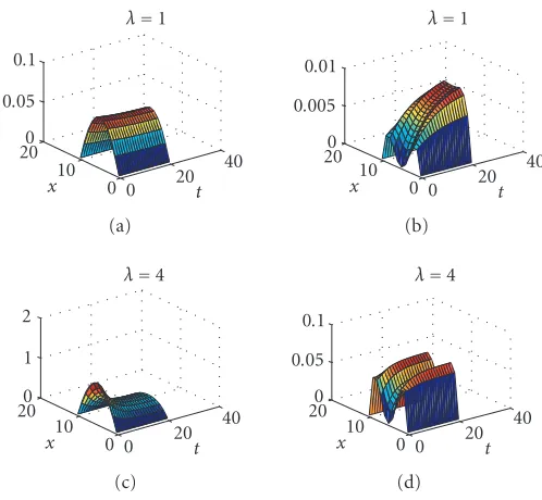
(c) 0 20 40 t 0 10 20 x 1 0 1

λ=4

(d)

15 10 ₅

x 0 10_t 20 30

0 2 4 6 8 10

4 λ=0.1

(a)

20 10

0

x 5 10 15 20 25

t

0 0.51 1.5

10

4 λ=0.1

(b)

15 10 ₅ 0

x 0 10 t20 30

0 0.01 0.02

λ=0.5

(c)

15 10 ₅ 0

x 0 10 t20 30

01 2 3 10 3 (d)

Figure 4.6. The lower solutionsw(x,t) andv(x,t) and the differencev(x,t)−w(x,t) for the slab ge-ometry, whenβ=0.5,δ=0.1, andλ=0.1, 0.5.

20 10

0

x ₀ 20_t 40

0 0.05 0.1

λ=1

(a)

20 10

0

x ₀ 20_t 40

0 0.005 0.01

λ=1

(b)

20 10

0

x ₀ 20_t 40

0 1 2

λ=4

(c)

20 10

0

x ₀ 20_t 40

0 0.05 0.1

λ=4

(d)

Figure 4.7. The lower solutionsw(x,t) andv(x,t) and the differencev(x,t)−w(x,t) for the slab ge-ometry, whenβ=0.5,δ=0.1, andλ=1, 4.

the right the difference between them. One can see that the two bounds are close to each other and for all values ofλwe havev≥w, that is, the lower solutionvis better thanw.

5. Concluding remarks

We have used comparison arguments to study a nonlinear parabolic equation arising from the theory of catalyst pellets reaction. For δβ≤1, a lower solution of the form w(x,t)=k(t)(φ1/φ1m) is obtained, whereφ1 is the first normalized eigenfunction of the associated Laplacian operator,φ1mis the maximum ofφ1inΩ, andk(t) is the solution of an IVP. Depending on the initial conditionk(0), the functionk(t) might be decreasing or increasing. An upper solution of the formu(x,t)=h(t)ψ(x) is obtained by solving a second-order linear IVP forh(t) and a linear PDE forψ, whereh(t) is increasing in time. The lower solution is used to give a sufficient condition for the solutionθto be increasing in time for certain initial condition. For the case whereδ >4 + 4/β, we have constructed a lower solutionw(x,t)=k(t)φ1(x), wherek(t) is increasing and depends on the value of λ∗_{. We present the upper and lower solutions for certain parameters in the three} geome-tries numerically. These upper and lower solutions are compared with the ones obtained by Pao [10] for the slab geometry.

References

[1] M. Al-Refai, Existence, uniqueness and bounds for a problem in combustion theory, Journal of Computational and Applied Mathematics 167 (2004), no. 2, 255–269.

[2] , Bounds and critical parameters for a combustion problem, Journal of Computational and Applied Mathematics 188 (2006), no. 1, 33–43.

[3] R. Aris, The Mathematical Theory of Diffusion and Reaction in Permeable Catalysts, Vol. I, Claren-don Press, Oxford, 1975.

[4] J. Bebernes and D. Eberly, Mathematical Problems from Combustion Theory, Applied Mathemat-ical Sciences, vol. 83, Springer, New York, 1989.

[5] D. W. Drott and R. Aris, Communications on the theory of diffusion and reaction—I: a complete parametric study of the first-order, irreversible exothermic reaction in a flat slap of catalyst, Chem-ical Engineering Science 24 (1969), no. 3, 541–551.

[6] A. K. Kapila and B. J. Matkowsky, Reactive-diffuse systems with Arrhenius kinetics: multiple solu-tions, ignition and extinction, SIAM Journal on Applied Mathematics 36 (1979), no. 2, 373–389. [7] , Reactive-diffusive system with Arrhenius kinetics: the Robin problem, SIAM Journal on

Applied Mathematics 39 (1980), no. 3, 391–401.

[8] A. K. Kapila, B. J. Matkowsky, and J. Vega, Reactive-diffusive system with Arrhenius kinetics: pe-culiarities of the spherical geometry, SIAM Journal on Applied Mathematics 38 (1980), no. 3, 382–401.

[9] M. L. Michelsen and J. Villadsen, Diffusion and reaction on spherical catalyst pellets: steady state and local stability analysis, Chemical Engineering Science 27 (1972), no. 4, 751–762.

[10] C. V. Pao, Nonlinear Parabolic and Elliptic Equations, Plenum Press, New York, 1992.

[12] D. H. Sattinger, Monotone methods in nonlinear elliptic and parabolic boundary value problems, Indiana University Mathematics Journal 21 (1972), no. 11, 979–1000.

Mohammed Al-Refai: Department of Mathematics and Statistics, Jordan University of Science and Technology, P.O. Box 3030, Irbid 22110, Jordan

E-mail address:m [email protected]

Qutaibeh Katatbeh: Department of Mathematics and Statistics, Jordan University of Science and Technology, P.O. Box 3030, Irbid 22110, Jordan