Path tracking algorithm for an autonomous ground robot

PATH TRACKING ALGORITHM FOR AN AUTONOMOUS GROUND ROBOT

NOORAIN BT MOHD JOHARY

A thesis submitted in

fulfillment of the requirement for the award of the Degree of Master of Electrical Engineering

FACULTY OF ELECTRICAL AND ELECTRONIC ENGINEERING UNIVERSITI TUN HUSSEIN ONN MALAYSIA

v

ABSTRACT

vi

ABSTRAK

vii

CONTENTS

TITLE PAGE

DECLARATION ii

DEDICATION iii

ACKNOWLEDGEMENT iv

ABSTRACT v

ABSTRAK vi

TABLE OF CONTENTS vii

LIST OF FIGURE x

LIST OF TABLE xi

LIST OF ABBREVIATIONS xii

LIST OF APPENDIX xiii

CHAPTER 1 INTRODUCTION

1.1 Project Background 1

1.2 Problem Statement 2

1.3 Objectives of the project 2

viii

CHAPTER 2 LITERATURE REVIEW

2.1 Introduction 4

2.2 Path Planning 5

2.3 Path Tracking 5

2.3.1 Kinematic Constraints 6 2.3.2 Dynamic Constraints 8

2.4 Previous Related Works 8

CHAPTER 3 METHODOLOGY

3.1 Introduction 16

3.2 Project Methodology Flowchart 17 3.2.1 Project Flowchart 18

3.3 Path Tracking 19

3.3.1 PID Controller 19 3.3.2 Characteristic of P, I, and D 21 Controller

3.3.2.1 Proportional Action 21 3.3.2.2 Integral Action 22 3.3.2.3 Derivative Action 22

3.4 Path Tracking Algorithm 23

3.5 Path Tracking Using PID Controller 23 3.6 Ground Robot Kinematic Modeling 25 3.7 Variable waypoint offset 27

3.8 MATLAB IDE 27

CHAPTER 4 RESULT AND ANALYSIS

4.1 Introduction 24

ix

Tracking Algorithm

4.2.1 Case 1 ₂₆ 4.2.1.1 Comparison between 36 Proportional, PD, and PID

Controller

4.2.2 Case 2 ₃₇ 4.2.2.1 Comparison between 37 No controller and Kinematic

Controller

4.2.2.2 Comparison between 38 Proportional, PD, and PID

Controller

4.2.3 Case 3 ₃₉ 4.2.3.1 Comparison between 39 No controller and Kinematic

4.2.3.2 Comparison between 40 Proportional, PD, and PID

Controller

4.3 Simulation with Different Value of 41 Tuning Factor

4.3.1 Case 1 ₄₂

4.4 Summary of the Chapter 50

CHAPTER 5 CONCLUSION

5.1 Conclusion 51

5.2 Recommendation 52

REFERENCES 53

x

LIST OF FIGURES

List Page

Figure 2.1 : Path planning configuration 5

Figure 2.2 : Definition of posture and velocities of two-wheeled mobile robot

7

Figure 3.1 : Methodology of project 17

Figure 3.2 : Flowchart of the project 18

Figure 3.3 : A block diagram of a PID controller in a feedback loop 19 Figure 3.4 : Definition of posture and velocities of car-like mobile robot 25

Figure 4.1 : Reference path 29

Figure 4.2 : Path tracking using No Controller 30

Figure 4.3 : Path tracking using kinematic controller 31 Figure 4.4 : Path tracked by proportional controller 32 Figure 4.5 : Path tracked by proportional-derivative controller 33 Figure 4.6 : Path tracked by proportional-integral-derivative controller 35 Figure 4.7 : Comparison between Proportional, PD and PID controller 36 Figure.4.8 : Comparison between No controller and Kinematic Controller 37 Figure.4.9 : Comparison between Proportional, PD, and PID controller 38 Figure.4.10 : Comparison between No controller and Kinematic Controller 40 Figure 4.11 : Comparison between Proportional, PD, and PID controller 41

Figure 4.12 : Path tracking with smaller 42

Figure.4.13 : Path tracking with larger 43

Figure 4.14 : Path tracking with smaller and 44

Figure.4.15 : Path tracking with larger and 45

Figure 4.16 : Path tracking with and is equal to 1 46

Figure 4.17 : Path tracking with best , , and 47

xi

LIST OF TABLE

List Page

Table 2.1 : List of Related Works 13

xii

LIST OF ABBREVIATIONS

PID - Proportional-Integral-Derivative VWO - Variable waypoint offset

WP - Waypoint

xiii

LIST OF APPENDIX

CHAPTER 1

INTRODUCTION

1.1 Project Background

2

use in close loop system. Among these features are its simple functionality and reliability.

1.2 Problem Statement

Most of path planning methods produce paths which consist of piece-wise linear segments. This in turn causes the paths have sharp corners, which are not feasible for mobile robot. While most of mobile robots are non-holonomic with kinematic and dynamic constraints, they are unable to traverse such paths. This needs the path to be smoothen considering the robots kinematic constraints such as minimum turning radius. Besides that, autonomous robot may experiences overshoot and deviation when following the path. Hence path smoothing or path tracking is needed to make the path satisfies the constraints. Therefore, path tracking algorithm for an autonomous ground robot need to be developed in order to ensure the robot are able to follow the reference path.

1.3 Objective

There are few objectives that need to be achieved at the end of this project. The objectives of this project are:

i. To propose a tracking algorithm for a car-like robot that can deal with very large tracking error.

ii. To implement tracking control algorithm so that the robot is able to track the planned path smoothly.

3

1.4 Project Scope

In order to achieve the objectives of the project, several scopes have been outline. The following are the scopes of the project.

i. Use a suitable algorithm and controller to keep the robot on track and follow the path smoothly.

ii. The robot is able to follow the existing planned path with less overshoot at every corner of path.

CHAPTER 2

LITERATURE REVIEW

2.1 Introduction

Literature review is a process of collecting and analyse data and information which are relevant to this study. The required data and information can be collected through variable sources such as journals, articles, reference books, online database and others. This chapter consists or two parts. The first part will be a case study on previous projects that relates to this project while the second part will focus on the theory aspects of this project.

2.2 Path Planning

5

defined constraint of the motion and decide the shortest path from the starting position to the target position.

2.3 Path Tracking

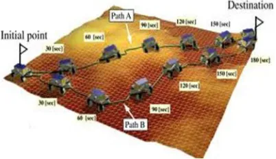
Path tracking in robotics is capabilities of the robots to follow the path that already exist with considering the motion smoothness or the dynamic constraints. Path tracking controller can be classified into four categories which is linear, non-linear, geometrical and intelligent approaches [1]. The linear approaches are computationally simple, but the path tracking motion is inconsistent with size of the path errors. To cope with the problem, several authors have proposed non-linear path tracking algorithm. Those include a path tracking method based on Lyapunov function [2, 3] and a non-linear steering control law [4] considering the driving speed. The non-linear approaches, however consider only path error convergence or system stability, but neglect the smoothness of the transient trajectory or dynamic constraints. The geometric approaches are considered as attempts to connect the path tracking to path planning. Tsugawa [7] has presented a target point following algorithm in which a cubic spline curve is used to determine the steering angle or rotational velocity of the robot. This geometric scheme show the smooth tracking motion to guide the mobile robot towards the reference path, but neglect the dynamic constraints, such as the curvature or acceleration limits which are important factors for avoiding robot or wheel slippage or stray away from the path.

6

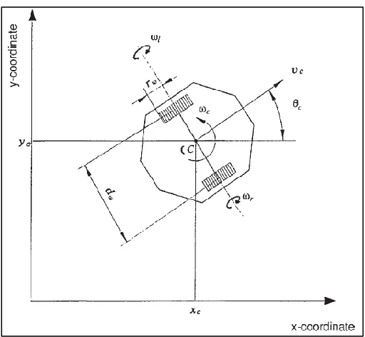
2.3.1 Kinematic Constraints

In this section, the error dynamic and kinematical constraints of robot are defined. For a mobile robot driven by two differential wheels, the center of motion, denoted by C is located at the midpoint between the left and right driving wheels. Assuming that the robot moves on the planner surface without slipping, the tangential velocity and angular velocity at the center C can be written as [1]

( ) ( )

( ) ( )

where and denote the rotational velocities of the right and left driving wheels, respectively, is the radius of the wheels, and is the azimuth length between the wheels. The kinematic equation of the mobile robot is given by

̇ ( )

̇ ( )

( )̇

7

(i) In case

_{[ ( ) ( )}

_{[ ( ) ( )}

_{( )}

(ii) In case

_{( ) ( )}

_{( ) (2.10)}

_(2.11)

where denotes the sampling index and is the sampling time

8

2.3.2 Dynamic Constraints

Any abrupt change in the robot motion may cause the slippage or mechanical damage to the mobile robot [1]. If the angular acceleration of each driving wheel is limited by ̇max

| ̇r,1| ̇max (2.12)

then, from (1) and (2), the tangential and angular accelerations of the robot are bounded by

| | | | ̇ (2.13)

The above equation means that the maximum allowable bounds on tangential and angular accelerations of the robot are coupled with each other. The ranges of each value to be independently considered are obtained by taking half the value of each maximum as

| | ̇ (2.14)

| | ̇

(2.15)

where and are the tangential and angular acceleration limits of the robot, respectively.

2.4 Related Work

9

K.C. Koh [1] has presented that dynamic constraints of the mobile robot should be considered in the design of path tracking algorithm. The driving velocity control law has been designed based on bang-bang control and the acceleration bounds of driving wheels need to be considered. The landing curve has been introduced as it works as an intermediate path smoothly steering the rotation of the robot towards the reference path. The target tracking algorithm used in this project is composed of two independent laws which is steering control law and velocity control law.

Sanhyuk [8] Park has studied the new guidance logic which is able to select a reference point on the desired trajectory and lateral acceleration command was generated by using the reference point. The several guidance logic have been developed which is the proportional derivatives controller (PD) has been used on the cross-track error, has an element of anticipation for the upcoming local desired flight path, and instantaneous vehicle speed was used in the algorithm. This kinematic factor adds an adaptive capability with respect to changes in vehicle inertial speed, due to the external disturbance.

Jeff Wit [9] has presented a new path tracking technique called ‘‘vector pursuit’’. This new technique is based on the theory of screws, which was developed by Sir Robert Ball in 1900. It generated a desired vehicle turning radius based on the vehicle’s current position and orientation relative to the position of a point ahead on the planned path and the desired orientation along the path at that point. The vector pursuit algorithm is compared to other geometrical approaches, and it is shown to be more robust, resulting in more accurate path tracking.

10

of an arc that a vehicle must follow to bring it from its current position to some goal position, where the goal is chosen as some point along the path to be tracked and the algorithm is extremely robust to poor sensing, poor actuation, combination with other control mechanisms, and is easily adapted for changing functionality. Another adjustable parameter has been implement is the radial tolerance that assigned to each waypoint. When the radial tolerance is set too low for the vehicle, the path is overshot at the corners. With a more realistic radial tolerance, the robot does not approach the waypoint itself as closely, but is able to adhere to the path more accurately.

R. Craig Conlter [11] has studied the implementation of the Pure Pursuit Path tracking Algorithm. The pure pursuit approached a method of geometrically determining the curvature that will drive the vehicle to a chosen path point, termed the goal point. The method itself is fairly straightforward. The only real implementation problems lie in deciding how to deal with the path information (communication, graphics, updating the path with new information from the planner). There is one parameter in the pure pursuit algorithm which is a lookahead distance. The effects of changing the lookahead distance must be considered within the problem faced such as regaining the path and maintaining the path.

Tao Dong [12] has presented path tracking and obstacle avoiding based on fuzzy logic approached. Fuzzy logic control algorithms are developed to achieve close path tracking while avoiding obstacles. The Fuzzy Logic Controller is activated when the obstacle sensor detects any obstacle. UAV velocity and heading angle change into corresponding different situations will be generated by the FLC. A two-layered FLC was used to make the UAV track its path while avoiding the fixed, but unexpected obstacles.

11

G. Ambrosino [14] has studied the path generation and tracking algorithm for 3D UAV. The 3D path has been obtained by using Dubins Algorithm. One of the characteristic of the path generated by the proposed algorithm is composed by straight lines and circles/arcs of constant radii. The line-of-sight guidance algorithm has been used for path tracking algorithm. This algorithm is based only on the kinematic equations of motion. The algorithm for the path tracking guarantees, under specified assumptions the tracking error, both in position and in attitude, asymptotically tends to zero.

Jacky Baltes [15] has presented the used of reinforcement learning in solving the path-tracking problem for car-like robots. The most important concept in reinforcement learning is the agent and environment. In the path tracking problem, the reward is based on how well the agent tracked the given path. Reinforcement learning can be adapted to control a car in path tracking. The controller is needed to keeps the car on the track. The reinforcement controller is the only controller that has been used successfully to drive cars with and without linear steering behaviour.

Takeshi Yamasaki [16] has studied about a guidance and control system for a trajectory-tracking unmanned aerial vehicle (UAV). A proportional navigation guidance law is applied to a trajectory-tracking flight to achieve the robust trajectory-tracking guidance and control system. The system employed a dynamic inversion technique for the guidance force generation, which allows the UAV to maintain high maneuverability, and a simple velocity control to obtain a desired velocity. With the proportional navigation guidance, UAV may avoid its control saturation or divergence even in large tracking-error situations.

12

stability of the control systems are analysed and proved using a Lyapunov stability theory.

A.Hemami [18] has proposed a new control strategy to determine the steering angle at each instant based on measured errors, the offset from the path and the deviation in orientation. The steering system is considered to control the angle of the steering wheel so that any deviation from the path is corrected in a stable manner and as fast as possible, and without oscillations about the path. Besides that, the dynamic equation of the vehicle is formulated to study the effect of a control strategy.

André KAGMA [19] has presented a method to track straight lines path with a car-like tricycle vehicle. Straight line tracking controller is used as a control strategy to track the pathas a robot is moves. The aim of this project is to design a controller which makes the vehicle follow the X – axis. Kinematics of the tricycle robot has been considered in this project.

13

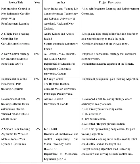
Table 2.1 shows the list of related works and project description that have been done before.

Table 2.1: List of Related Works

Project Title Year Author Project Description

Path-tracking Control of

Non-holonomic Car-like

Robot With

Reinforcement Learning

- Jacky Baltes and Yuming Lin

Centre for image Technology

and Robotics University of

Auckland, Auckland New

Zealand.

-Used reinforcement Learning and Reinforcement

Controller.

A Simple Path Tracking

Controller For

Car-Like Mobile Robots

- André Kamga and Ahmed

Rachid

System automatic Laboratory

France.

-Design and used straight line tracking controller

as a control strategy to track the path.

-Consider kinematic of the tricycle robot.

A New Control Strategy

for Tracking in Mobile

Robots and AGV’s

1990 A. Hemami, M.G. Mehrabi,

and R.M.H. Cheng

Department of Mechanical

Engineering Concordia

University, Canada

-Proposed a new control strategy that considers

steering system.

-Formulated dynamic equation of the vehicle.

Implementation of the

Pure Pursuit Path

tracking Algorithm

1992 R. Craig Conlter

The Robotics Institute

Camegie Mellon University

Pittsburgh, Pennsylvania

-Implement pure pursuit path tracking Algorithm.

Development of path

tracking software for an

autonomous

steered-wheeled robotic vehicle

and its trailer

1997 Arturo L.Rankin

University of Florida

-Developed a path following strategy where

accuracy is easily attained

-Used three types of steering control

1.PID Controller

2.Pure pursuit control

3.Weighted PID/pure pursuit solution

A Smooth Path Tracking

Algorithm for Wheeled

Mobile Robots With

Dynamic Constraints

1999 K. C. KOH

Division of mechanical and

control engineering Sun

Moon University Korea

H. S. CHO

Department of Mechanical

Engineering, KAIST

-Used time optimal bang-bang control for path

tracking algorithm.

-Introduced a landing curve so that mobile robot

could softly land on the target line.

-Target tracking algorithm used is steering

14

Autonomous Ground

Vehicle Path Tracking

2000 Jeffrey S. Wit

University of Florida

-Used vector pursuit tracking technique.

Tracking Control of a

Mobile Robot Using

Neural Dynamics Based

Approaches

2001 Guanfeng Yuan

The Faculty of Graduate

Studies of The University of

Guelph

-Used backstepping techniques and a neural

dynamics model.

- The stability of the control systems are analysed

using a Lyapunov

Path Planning And

Tracking in a 3D

Complex Environment

for an Anthropomorphic

Biped Robot

2002 Jean – Matthieu Bourgeot,

Nathalie Cislo, Bernand

INRIA Rhone-Alpes, BIP

Project, Montbonnot, France.

-3D path planning method develop by using A*

algorithm.

- Path tracking strategy measure heading and

literal offset.

A new nonlinear

Guidance Logic for

Trajectory Tracking.

2004 Sanhyuk Park, John Deyst

and Jonathan P.How

Massachusetts Institute of

Technology, Cambridge,

MA,USA

-Used proportional derivative (PD) controllers.

-Three purposes angle used in the guidance

logic

1. Provides a heading correction

2. Provides PD control on cross track

3. Provides an anticipatory acceleration command

to exactly follow a circular reference trajectory.

-Used instantaneous vehicle speed in the

algorithm.

Path Tracking for

Unmanned Ground

Vehicle Navigation

2005 J. Giesbrecht, D. Mackay, J.

Collier, S. Verret DRDC

Suffield Defence Research

and Development Canada

-Usedpure pursuit algorithm.

-Implement the radial tolerance waypoints.

Path Tracking and

Obstacle Avoidance of

UAVs - Fuzzy Logic

Approach

2005 Tao Dong, X. H. Liao, R.

Zhang, Zhao Sun and Y. D.

Song

Department of Electrical and

Computer Engineering

North Carolina A&T State

University, USA

-Used fuzzy logic based approach to path

tracking and obstacle avoiding.

-Used fuzzy logic controller.

Algorithms for 3D UAV

Path Generation and

Tracking

2006 G. Ambrosino, M. Ariola, U.

Ciniglio, F. Corraro, A.

Pironti and M. Virgilio

Proceedings of the 45th IEEE

Conference on Decision &

Control USA,

-Used Dubins Algorithm for 3D Path.

-Used line-of-sight guidance algorithm for

15

Robust

Trajectory-Tracking Method for

UAV Guidance

Using Proportional

Navigation

2007 Takeshi Yamasaki, Hirotoshi

Sakaida, Keisuke Enomoto,

Hiroyuki Takano and Yoriaki

Baba

Department of Aerospace

Engineering, National

Defense Academy,

Kanagawa, Japan

-Used proportional navigation guidance law.

-Employed a dynamic inversion technique for

the guidance force generation.

CHAPTER 3

METHODOLOGY

3.1 Introduction

This chapter will describe the overall process to develop this research project, method and technique approach to complete the project. To accomplish it successfully, the method and technical strategy implied is the most important disciplined need to be concerned.

3.2 Project Methodology Flowchart

17

Figure 3.1: Methodology of Project

Start

Research & Literature Review

Planning and select suitable controller and algorithm

Write program for the robot path tracking by using Matlab software

Test

Modify the program

End Ok

Yes

18

3.2.1 Project flowchart

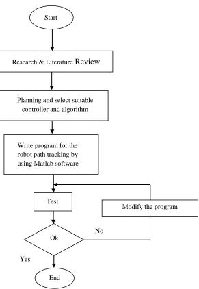
Figure 3.2 shows the flow chart for this project. It consist of the process to tracking the path by considering the prior information and path tracking algorithm is applied in order to track the existing path. Path tracker is realised using controllers to keep the robot on track and reduce the overshoot or deviation when following the path.

Figure 3.2: Flowchart of the project Start

End Prior information:

 Starting point

 Target point

 Existing path

Apply path tracking algorithm & path tracker is realized using controller

Tracking path?

Yes

19

3.3 Path Tracking

Path tracking is a capability of robot to follow the existing or reference path with respect to the path and path information. Path tracking is an important issue and one of the most fundamental problems in mobile robots. The purpose of path tracking is to follow the planned path smoothly by considering the kinematic and dynamic constraint. Therefore the controller is needed which keep the robot on track and reduce the overshoot or deviation when following the path.

3.3.1 PID Controller

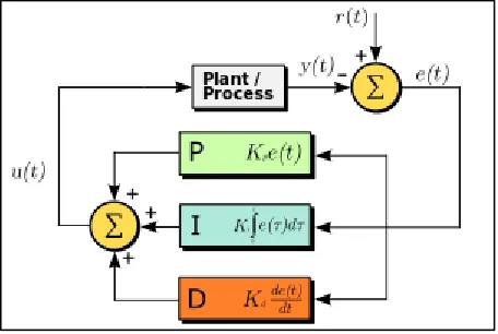
A proportional-integral-derivative controller (PID controller) is a generic control loop feedback mechanism (controller) widely used in industrial control systems. A PID controller calculates an "error" value as the difference between a measured process variable and a desired set point. The controller attempts to minimize the error by adjusting the process control inputs.

The PID controller calculation algorithm involves three separate constant parameters, and is accordingly sometimes called three-term control: the proportional, the integral and derivative values, denoted P, I, and D. Simply put, these values can be interpreted in terms of time: P depends on the present error, I on the accumulation of past errors, and D is a prediction of future errors, based on current rate of change.

20

The PID algorithm is described by

( ) ( ) ∫ ( )

( )

where y is the measured process variable, r the reference variable, u is the control signal and is the control error . The reference variable is often called the set point. The variable ( ) represent the tracking error, the difference between the desired input value ( ) and the actual output( ). This error signal ( ) will be sent to the PID controller, and the controller computes both the derivative and the integral of this error signal. The control signal ( ) to the plant is equal to the proportional gain ( ) times the magnitude of the error plus the integral gain ( ) times the integral of the error plus the derivative gain ( ) times the derivative of the error.

This control signal ( ) is sent to the plant, and the new output ( ) is obtained. The new output ( ) is then fed back and compared to the reference to find the new error signal ( ). The controller takes this new error signal and computes its derivative and its integral again until the output obtain is satisfied. The control signal is thus a sum of three terms, the P-term (which is proportional to the error), and the I-term (which is proportional to the integral of the error), and the D-term (which is proportional to the derivative of the error). The controller parameters are proportional gain Kp, integral time

Ti, and derivative time Td.

The transfer function of a PID controller is found by taking the Laplace transform of Eq. (1).

( )

= Proportional gain = Integral gain

21

3.3.2 Characteristic of P, I, and D controllers

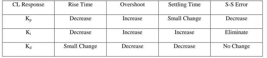
A proportional controller ( ) will have the effect of reducing the rise time and will reduce but never eliminate the steady-state error. An integral control ( ) will have the effect of eliminating the steady-state error for a constant or step input, but it may make the transient response slower. A derivative control ( ) will have the effect of increasing the stability of the system, reducing the overshoot, and improving the transient response. The effects of each of controller parameters and on a closed-loop system are summarized in the table below.

Table 3.1: Effects of each of controller parameters

CL Response Rise Time Overshoot Settling Time S-S Error

Kp Decrease Increase Small Change Decrease

Ki Decrease Increase Increase Eliminate

Kd Small Change Decrease Decrease No Change

These correlation may not be exactly accurate, because and are dependent on each other. In fact, changing one of these variables can change the effect of the two other. The table should only be used as a reference when determining the values for and .

3.3.2.1 Proportional Action

The proportional term produces an output value that is proportional to the current error value. The proportional response can be represents as per equation below:

Where

( )

Pout: Proportional term of output

Kp: Proportional gain, a tuning parameter e: Error = SP − PV

22

t: Time or instantaneous time (the present)

3.3.2.2 Integral Action

The contribution from the integral term is proportional to both the magnitude of the error and the duration of the error. Summing the instantaneous error over time (integrating the error) gives the accumulated offset that should have been corrected previously. The accumulated error is then multiplied by the integral gain and added to the controller output [10]. The magnitude of the contribution of the integral term to the overall control action is determined by the integral gain, Ki. The integral term is given by:

( )

Where

Iout: Integral term of output

Ki: Integral gain, a tuning parameter e: Error = SP − PV

: Time in the past contributing to the integral response

3.3.2.3 Derivative Action

The rate of change of the error is calculated with respect to time, multiplied by another constant D, and added to the output. The derivative term is used to determine a controller's response to a change or disturbance of the process. The derivative term is given by:

( )

where

Dout: Derivative term of output

(3.4)

23

K_d: Derivative gain, a tuning parameter e: Error = SP − PV

t: Time or instantaneous time (the present)

3.4 Path Tracking Algorithm

To achieve the project goal in well-organized manner, the actual algorithm is implemented as follows.

Current point Previous point ̇ Course rate change

Current steering angle Previous steering angle Maximum steering angle ̇ Maximum steering rate Difference between the and Sampling Time

1. Find ground robot course angle from current point, to the next waypoint. 2. Calculate the difference between the previous ( ) and current point, 3. Calculate course rate change, ̇ : ̇ = ( )

4. Calculate current steering angle,

5. Calculate the difference, between the previous steering angle, and . 6. If > ̇ , set = ̇ .

24

3.5 Path Tracking Using PID Controller

In the PID Controller, the control law is determined based on the following errors: (i) Heading error, ψerr. (ii) Cross-track error, Yerr.

The reference heading angle is calculated from two consecutive waypoints WP of the initial path:

₍₍

) (( )) j and j − 1 are the current and previous waypoint indexes within which the path is calculated.

The actual heading angle of the path is derived using the previous and current positions. ₍₍

) ( ))

ψerr is calculated from the difference between the reference heading angle, ψref and the

current actual heading angle, ψk.

Also, the shortest distance from actual position to the reference path, Yerr is needed to design the controller for robot and can be calculated using linear equation. From ψerr and Yerr, a control law using PID controller is then formulated to regulate the current path state. P term in PID controller is defined as

with KP1 and KP2 are the proportional gains. The I term is

( ( ) ( )) ( ( ) ( ))

The D term is

REFERENCES

[1] K. C. Koh and H. S. CHO, A Smooth Path Tracking Algorithm For Wheeled Mobile Robots With Dynamic Constraints, Journal Of Intelligent And Robotics System (1999) 24: 367-385.

[2] Hemami, A., Mehrabi, M. G., and Cheng, R. M.: Synthesis For An Optimal Control Law For Path Tracking In Mobile Robots, Automatica 28(2) (1992), 383–387.

[3] Kanayama, Y., Kimura, Y., Miyazaki, F., and Noguchi, T.: A Stable Tracking Control Method for an Autonomous Mobile Robots, in: Proc. of the IEEE Internat. Conf. on Robotics and Automation, (1990), pp. 384–389.

[4] Hemami, A., Mehrabi, M. G., and Cheng, R. M.: A New Strategy for Tracking in Mobile Robots and AGV’s, in: Proc. of the IEEE Internat. Conf. on Robotics and Automation, (1990), pp. 1122–1127.

[5] Elnagar, A. and Basu, A.: Piecewise Smooth and Safe Trajectory Planning, Robotica 12 (1994), 299–307.

[6] Tounsi, M. and Le Corre, J. F.: Trajectory Generation for Mobile Robots, Mathematics and Computers in Simulation, 1996, pp. 367–376.

[7] Tsugawa, S. and Murata, S.: Steering Control Algorithm for Autonomous Vehicle, in: Proc. of the Japan-USA Symp. on flexible automation, (1990), pp. 143–146.

[8] Sanhyuk Park, John Deyst and Jonathan P.How.: A new nonlinear Guidance Logic for Trajectory Tracking, Massachusetts Institute of Technology, Cambridge, (2004) MA, 02139, USA

54

[10] J. Giesbrecht, D. Mackay, J. Collier, S. Verret: Path Tracking for Unmanned Ground Vehicle Navigation, DRDC Suffield Defence Research and Development Canada (2005).

[11] R. Craig Conlter.: Implementation of the Pure Pursuit Path tracking Algorithm, The Robotics Institute Camegie Mellon University Pittsburgh, Pennsylvania (1992).

[12] Tao Dong, X. H. Liao, R. Zhang, Zhao Sun and Y. D. Song.: Path Tracking and Obstacle Avoidance of UAVs - Fuzzy Logic Approach Department of Electrical and Computer Engineering, North Carolina A&T State University, USA (2005).

[13] J.Matthieu Bourgeot, Nathalie Cislo, Bernand.: Path Planning And Tracking in a 3D Complex Environment for an Anthropomorphic Biped Robot, ( 2002) INRIA Rhone-Alpes, BIP Project, Montbonnot, France.

[14] G. Ambrosino, M. Ariola, U. Ciniglio, F. Corraro, A. Pironti and M. Virgilio.: Algorithms for 3D UAV Path Generation and Tracking, Proceedings of the 45th IEEE Conference on Decision & Control (2006) USA.

[15] Jacky Baltes and Yuming Lin.: Path-tracking Control of Non-holonomic Car-like Robot with Reinforcement Learning, Centre for image Technology and Robotics University of Auckland, Auckland New Zealand.

[16] Takeshi Yamasaki, Hirotoshi Sakaida, Keisuke Enomoto, Hiroyuki Takano and Yoriaki Baba.: Robust Trajectory-Tracking Method for UAV Guidance Using Proportional Navigation Department of Aerospace Engineering, National Defense Academy, Kanagawa, Japan (2007).

[17] Guanfeng Yuan.: Tracking Control of a Mobile Robot Using Neural Dynamics Based Approaches The Faculty of Graduate Studies of The University of Guelph (2001).

55

[19] André Kamga and Ahmed Rachid.: A Simple Path Tracking Controller for Car-Like Mobile Robots, System automatic Laboratory France.

[20] Arturo L.Rankin.: Development of path tracking software for an autonomous steered-wheeled robotic vehicle and its trailer, University of Florida (1997). [21] K. Astrom and T. Hugglund(1995), Controllers: Theory, Design and Tuning, 2nd