Discounted Generalized Transportation Problem

Discounted Generalized Transportation Problem

Debiprasad Acharya

, Manjusri Basu

and Atanu Das

*

Department of Mathematics; N. V. College; Nabadwip; Nadia; W.B.; India.

**

Department of Mathematics; University of Kalyani; Kalyani - 741235; India.

Abstract- In generalized transportation problem(GTP), the cost of transportation cij per unit product from the i

th

origin to the jth destination is considered as independent of amount of transported commodity xij. But in real life problems, there are many

situations, e.g. quantity discount, price break etc., in which cost of transportation cij depends upon the amount of transported

commodity xij. Based on these situations, in this paper, we

consider a new type of discounted generalized transportation problem in which the cost of transportation cij per unit product

depends on the amount of transported commodity xij. Thereby,

we develop a new algorithm for obtaining the optimum solution of this problem. Finally, a numerical example is illustrated to support the algorithm.

Index Terms- Generalized transportation problem, Step function, Discount, Discounted generalized transportation problem

I. INTRODUCTION

itchcock [15] was pioneer of the basic transportation problem, Dantzig [13], Charnes and Cooper [11], Appa [1] developed further. Now a days, there are several procedures to solve the transportation problems. Arsham and Khan [2] considered simplex-type algorithm for general transportation problems. Basu et. al. [7,8,9] considered different types of transportation problems.

But in real life, there are many situations, e.g. quantity discount, price breaks etc. where the transportation cost may not be linear. Non linearity depends upon the character of the objective function as well as the character of the constraints. Cooper and Dredes [12] considered an approximate solution method for the fixed charge problem. Bhatia et. al. [10] considered time-cost trade-off in a transportation problem. Klingman and Russel [16] considered solving constrained transportation problems. Thirwani [17] considered fixed charge bi-criterion transportation problem with enhanced flow.

There are many business problems, industrial problems, machine assignment problems, routing problems, etc. that have

the characteristics in common with generalized transportation problem that has been studied by several authors. Balas and Ivanescu [4] introduced on the generalized transportation problem. Balachandrana and Thompson [3] considered an operator theory of parametric programming for the generalized transportation Problem. In 1987, Hadley [14] gave the detailed solution procedure for solving generalized transportation problem. Basu and Acharya [5,6] considered different types of generalized transportation problem.

Day by day, the importance of discounted generalized transportation problem is increasing practically in a great deal, but the method for finding the optimum solution of this kind of generalized transportation problems, however, lacks of the desired attention.

There are several differences between classical transportation problem and generalized transportation problem which are given as follows:

1. The rank of the co-efficient matrix of [xij]mn in

generalized transportation problem is (m+n), where as in classical transportation problem it is (m+n – 1)

2. In generalized transportation problem the value of xij may

not be integer though it must be integer in classical transportation problem.

3. The activity vector in generalized transportation problem is pij = dij ei + em+j, where dij = positive constants rather than

unity.

Where as in classical transportation problem it is given by pij = ei + em+j.

4. In generalized transportation problem, it need not be true that cells corresponding to basic solution form a tree.

5. In generalized transportation problem that =

is not necessary.

In this paper we develop a new algorithm to find the solution of discounted generalized transportation problem where the cost function is taken as step function. Thereby we illustrate this problem numerically.

II. PROBLEM FORMULATION

Let the discounted generalized transportation problem consists of „m‟ origins and „n‟ destinations, where xij = the amount of product transported from the ith origin to the jth destination,

cij = the cost involved in transporting per unit product from the i th

origin to the jth destination, ai = the number of units available at the origin i,

bj = the number of units required at the destination j,

dij = positive constants rather than unity.

(1)

subject to, ; for i=1,2,3,……….,m. (2)

; for j = 1,2,3,……….,n. (3)

and (4)

where > > > ………. > and xij  0. Net Evaluation Introducing slack variables, the problem P1 can be written as (5)

subject to, ; for i = 1,2,3,……….,m. (6)

; for j = 1,2,3,……….,n,n+1. (7)

where dij=positive constants rather than unity, xij  0 for all (i,j), and the values of cij are given in (4). Let ui (1 i  m) and vj (1 j  n+1) be the dual variables. So that, dijui + vj = cij for 1 I  m, 1 j  n. ui = 0 for 1 I  m, j = n + 1. (8)

where ui, vj are unrestricted for all (i,j). Now for any standard Primal L.P.P. with basis B and associated cost vector cB, the associated solution to its dual problem WB, is given by WB = cB B -1 . Thus, if pj is the j th column of the primal constraint matrix, then an expression for evaluating the net-evaluation for minimization problem is given by Zj – cj = cB ( B-1 pj ) – cj (9)

= WB pj – cj  j. But, in the present case of rectangular transportation problem, the dual solution can be represented by (u,v) = ( u1,u2, ……, um,v1,v2, ………, vn ) and therefore the net evaluations are analogously obtained by simply replacing cj  cij, WB  (u,v), pj  pij in the above formula. Thus we have the net evaluation as: Zij – cij =(u,v) pij – cij =( u1,u2,….., um,v1,v2,…….,vn ) [ dijei + em+j] – cij (10)

=( dij ui + vj ) – cij for i=1,2,……..,m; j=1,2,………,n+1. where pij(= dijei+em+j) is the column vector of the constraint matrix associated with the rectangular variable xij. For simplicity, we shall denote the net evaluation Zij – cij by ij in all our further discussion. Theorem: A solution of the discounted generalized transportation problem will be feasible solution if for any cell (q,r), xqr < (xqr + yqr), where 1 k<l  g also yqr>0 and > for 1 q  m, 1  r  n. Proof: Let Z1 be the total cost and F1 be the total flow where (q,r) be one of its allocated cell and xqr be its allocation where ( < xqr  ). Then (11)

Also let Z2 be the total cost and F2 be the total flow if (xqr + yqr) where < xqr + yqr  , be allocated at the (q,r) cell and all

other allocations are same as in flow F1. Therefore

(13)

and where < (xqr +yqr ) (14)

Obviously F1 + yqr > F1 where < (xqr +yqr )

Let us assume that the given condition xqr> (xqr+yqr) does not hold. Then

Z1 – Z2 = xqr – cqr (xqr + yqr )  0; => Z_1 > Z_2

But F2 > F1; So Z1 > Z2 => F1 < F2, which is a contradiction.

So, our assumption is wrong. Hence the theorem.

III. ALGORITHM

Step 1. Find the initial solution with the associated cost vector and the corresponding cost Z1 by using North West Corner Rule.

Step 2. Set r=1.

Step 3. Write with the associated vector and corresponding cost Zr. Step 4. Calculate dual variables ui (1  i  m) and vj (1  j  n).

Step 5. Calculate net evaluation ij  (i,j)  B. If ij  0  (i,j)  B. Then go to step 10.

Step 6. Calculate st = Max {ij : ij > 0 }. Then (s,t) cell enters into the basis.

Step 7. Let ; 1 i  m.

; 1 j  n+1.

where pst=dst es + em+t. After determining we calculate

Then (k,l) cell leaves the basis.

Step 8. The improved solution is for (i,j)B and (i,j)  (s,t) = for (i,j) = (s,t)

Step 9. Set r=r+1, goto step 3.

Step 10. Write the optimum solution is X*= with the associated cost vector = and the minimum cost is Z* = Zr. Step 11. Stop.

IV. NUMERICAL EXAMPLE

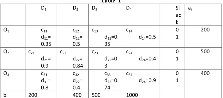
We consider the following problem given in Table 1

Table 1

D1 D2 D3 D4 Sl

ac k

ai

O1 c11

d11=

0.35

c12

d12=

0.5 c13

d13=0.

35

c14

d14=0.5

0 1

200

O2 c21

d21=

0.9 c22

d22=

0.84 c23

d23=0.

3

c24

d24=0.4

0 1

500

O3 c31

d31=

0.8

c32

d22=

0.4

c33

d23=0.

74

c34

d24=0.9

0 1

400

The variable costs are given below:

c11 = 203 if 0  x11 100 c12 = 401 if 0  x12  100

= 201 if 100 < x11  150 = 400 if 100 < x12  300

= 200 if x11>150 = 399 if x12>300

c13 = 400 if 0  x13 150 c14 = 751 if 0  x14  400

= 399 if 150 < x13  350 = 750 if 400 < x14  700

= 398 if x13>350 = 749 if x14>700

c21 = 502 if 0  x21 100 c22 = 604 if 0  x22  100

= 500 if 100 < x21  150 = 600 if 100 < x22  300

= 498 if x21>150 = 599 if x22>300

c23 = 602 if 0  x23 200 c24 = 752 if 0  x24  350

= 600 if 200 < x23  400 = 750 if 350 < x24  600

= 599 if x23>400 = 749 if x24>600

c31 = 401 if 0  x31 100 c32 = 502 if 0  x32  150

= 400 if 100 < x31  150 = 500 if 150 < x32  300

= 398 if x31>150 = 499 if x32>300

c33 = 602 if 0  x33 200 c34 = 901 if 0  x34  500

= 600 if 200 < x33  350 = 900 if 500 < x34  750

= 599 if x33>350 = 899 if x34>750

Applying step 1, we get the following result in Table 2

Table – 2

D1 D2 D3 D4 Slack ai

O1 200

200 0.35

400 260 0.5

400

0.35

751

0.5

0

1

200

O2 502

0.9

600 140 0.84

599 500 0.3

750 581 0.4

0

1

500

O3 398

0.8

502

0.4

599

0.74

901 419 0.9

0

22.9 1

400

bj 200 400 500 1000

Applying step 2, set r=1.

Applying step 3, we get = {x11 = 200, x12 = 260, x22 = 140, x23 = 500, x24 = 581, x34 = 419, x3S = 22.9} with the associated

cost vector = {c11 = 200, c12 = 400, c22 = 600, c23 = 599, c24 = 750, c34 = 901, c3S = 0} and the corresponding cost Z1 = 1340769.

Applying step 4, we get dual variables are u1=  1034.2, u2=377.5, u3=0, v1=561.97, v2=917.1, v3=712.25 and v4=901.

Applying step 5, we get the values of ij  (i,j)  B are 13 = 49.72, 14 = 367.1, 1S =1034.2, 21 = 275.78, 2S = 377.5,

31 = 163.97, 32 = 415.1 and 33 = 113.25.

Applying step 6, we get st = Max {163.97, 415.1, 113.25 } = 415.1 at (3,2) cell. Therefore (3,2) cell enter into the basis.

Applying step 7, we get the values of are =0, =0, =1, =0, =2.1, =2.1 and =1.49.

 = min { 140, 199.5} =140 = . Therefore (2,2) cell leaves the basis.

Applying step 8, we get the values of are =200, = 260, =500, =875, =140, =125, =231.5 and tabulated in Table 3.

Table – 3

D1 D2 D3 D4 Slack ai

O1 200

200 0.35

400 260 0.5

399

0.35

751

0.5

0

1

200

O2 502

0.9

600

0.84

599 500

750 875

0

1

0.3 0.4

O3 398

0.8 502 140 0.4 602 0.74 901 125 0.9 0 231.5 1 400

bj 200 400 500 1000

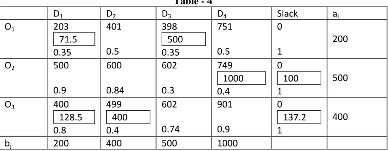
Applying step 9, set r = r + 1 and go to Step 3. The values of with the associated cost vector give in Table 3 and the corresponding cost Z2=1281780. Proceeding in this way the final table given by Table 4.

Table - 4

D1 D2 D3 D4 Slack ai

O1 203

71.5 0.35 401 0.5 398 500 0.35 751 0.5 0 1 200

O2 500

0.9 600 0.84 602 0.3 749 1000 0.4 0 100 1 500

O3 400

128.5 0.8 499 400 0.4 602 0.74 901 0.9 0 137.2 1 400

bj 200 400 500 1000

Applying step 10, the optimum solution is X*={ x11= 71.5, x13=500, x24=1000, x31=128.5, x32=400 }, with the associated cost

vector ={c11=203, c13=398, c24=749, c31=400, c32=499 } and the optimum cost Z*= 1213514.5

REMARK:

If we consider the problem

subject to, ; for i = 1,2,3,……….,m.

; for j = 1,2,3,……….,n.

where the values of cij are given in equation (2.4), and xij  0 (1  i  m, 1  j  n).

Then this problem (P1) can easily be converted to our proposed problem (P1) by transformation =wij for (1  i  m, 1

 j  n);

REFERENCES

[1] G. M. Appa, “The transportation problem and its variants,” Operational Research Quarterly, 1973, p.p. 79 – 99.

[2] H. Arsham and A. B. Kahn, “A simplex-type algorithm for general transportation problems: An alternating to stepping-stone,” Journal of Operational Research Society, 1989, p.p. 581 – 590.

[3] V. Balachandrana and G. L. Thompson, “An Operator Theory of Parametric Programming for the Generalized Transportation Problem-II: Rim, Cost and Bound Operators,” Naval Res. Log. Quart, 1975, p.p. 101 – 125.

[4] E. Balas and P. L. Ivanescu, “On the generalized transportation problem,” Management Science, 1964, p.p. 188 – 202.

[5] M. Basu and D. Acharya, “An algorithm for the optimum time-cost trade-off in generalized solid transportational problem,” International Management System, 2000, p.p. 237 – 250.

[6] M. Basu and D. Acharya, “On quadratic fractional generalized solid bi-criterion transportation problem,” An International Journal of Mathematics & Computing, 2002, p.p. 131 – 143.

[7] M. Basu, D. Acharya and A. Das, “The algorithm of finding all paradoxical pair in a linear transportation problem,” Discrete Mathematics, Algorithm and Application, 2012, 1250049 (9pages), World Scientific Publising Company, DOI: 10.1142/S1793830912500498.

[8] M. Basu, B. B. Pal and A. Kundu, “An algorithm for the optimum time-cost trade-off in three dimensional transportational problem,” Optimization, 1993, p.p. 177 – 185.

[9] M. Basu, B. B. Pal and A. Kundu, “An Algorithm For The Optimum Time Cost Trade-off in Fixed Charge Bi-criterion Transportation Problem,” Optimization, 1994, p.p. 53 – 68.

[10] H. L. Bhatia, K. Swarup and M. Puri, “Time-cost trade-off in a transportation problem,” Opsearch, 1976, p.p. 129 – 142.

[11] A. Charnes and W. W. Cooper, “The stepping stone method of explaning linear programming calculations in transportation problems,” Management Science, 1954, p.p 49 – 69.

[12] L. Cooper and C. Dredes, “An approximate solution method for the fixed charge problem,” Naval Research Logistics Quarterly, 1967, p.p 101 – 113. [13] G. B. Dantzig, Linear Programming and Extensions (Princeton University

Press, NJ, 1963).

[14] G. Hadley, Linear Programming, Narosa Publishing House, New Delhi, 1987.

[15] F. L. Hitchcock, “The distribution of a product from several resources to numerous localities,” Journal of Mathematical Physics, 1941, p.p 224 – 230. [16] D. Klingsman and R. Russel, “Solving Constrained Transportation

Problems,” Operations Research, 1975, p.p. 91 – 105.

AUTHORS

First Author – Debiprasad Acharya,Department of

Mathematics; N. V. College; Nabadwip; Nadia; W.B.; India., Email:[email protected]

Second Author – Manjusri Basu, Department of Mathematics;

University of Kalyani; Kalyani - 741235; India, Email: [email protected]

Third Author – Atanu Das, Department of Mathematics;