Bayesian Ecometrics – A genial device to ponder Ecological Data Analysis

Bayesian Ecometrics – A genial device to ponder

Ecological Data Analysis

Subbiah, M

, Kamal Nasir, V

, Srinivasan, M.R

, Naveed, MS

Department of Mathematics, L.N Government College, Ponneri, India **

Department of Mathematics, The New College, Royapettah, Chennai, Tamil Nadu, India ***

Department of Statistics, University of Madras, Chennai, Tamilnadu, India ****

Department of Zoology, The New College, Royapettah, Chennai Tamil Nadu, India

Abstract- Bayesian statistics is becoming an important statistical tool for practitioners to deal with analysis of complex data and complicated statistical models. The impact of Bayesian analysis in combination with Markov Chain Monte Carlo (MCMC) technology is realized optimally in the domain of applications. The ecological data could be a storehouse of natural history and experimental data is used to address hidden uncertainty. Bayesian inference could be the most straightforward and natural way of analyzing and interpreting the related ecological hypotheses. This study basically aims to exploit the inbuilt advantages of Bayesian approach in studying the prevalence of Meiofaunal population from the data collected at five different (Pulicat, Royapuram, Napier, Marina, Adyar) coastal areas of Chennai, India.

Index Terms- Bayesian methods, MCMC, Meiofauna, Sparseness, WinBUGS

I. INTRODUCTION

tatistics has a significant and unique characteristic that has been influenced largely by many other sciences with which it could interact. The list of other faculties include an extensively large number of areas such as atmospheric, bio medical, economic sciences, ecological, educational, psychological, public health, market research and many more. Most or all these studies could provide an ample scope for statistical intervention or contribution with their objective and vast array of data in high dimensional or hierarchical methods.

The challenges in data analysis has also been faced and during these kind of interventions, yet the powerful advanced computational developments lead or assist statistics into a greater and broader purview of data modeling and effective and meaningful interpretations. It is also to point out that with a visible better growth in the communication between statistics and other disciplines of science, a scope in incorporate subject matter, experts‟ opinion has been increased in many data analyses and model building. Piegorsch et al (1998) have observed this twin advantage as an upward spiral so that science and society could benefit with the interactions of disciplines. Statistic in a wider perspective could be classified as long run frequentist and Bayesian paradigms. A lot of conceptual and computational difference exists between these two methodologies; however this work does not intend to compare or contrast the two procedures. The principle aim of the paper is to have a broader outline of three fold aspects; building the theory,

computations and an application specifically to an ecological study. As recent decades could witness a surge in the application of Bayesian statistics and many researchers have pointed out the advantages from model formulation to interpretation of the results, this present work could be considered as another application of Bayesiansim to a more complicated study in that usual “log run” or “identical sample” assumptions might not hold apparently.

The paper has been organized as follows; section 2 lists recent and appropriate Bayesian literature pertains in particular to many ecological data. Section 3 covers a quick overview of conceptual and computational aspects of Bayesian statistics. The ecological data that has been considered for the present study is elaborated in section 4. An illustrative data analysis has been presented in section 5 and concluding remarks in section 6.

II. BAYESIANSATWORK

From the mid 20th century, with the availability of fast, accurate and affordable computing algorithms and machines, Bayesian approach could find a large scale applications in many fields from agriculture to business; medicine to social psychological studies; education to economics. However, this work aims in presenting a few yet more reasonable list of literature in environmental, ecological or generally bio scientific studies. Stephans et al (2006) have pointed out the way ecologists and evolutionary biologists who deal with high natural variability system and dependence of statistical procedure for their inference.

A chronological sequence of articles could provide many interesting applications of Bayesian methods ranging from parameter estimations to linear model to meta-analysis. As noted earlier. Piegorsch et al (1998) have discussed some selected applications of statistical theory to environmental sciences that include atmospheric pollution, mortality analysis, space-time modeling of acid rain, ecological monitoring and assessment and animal populations. Gurevitch and Hedges (1999) have elaborated the methods for the meta-analysis of ecological data that include fixed vs mixed models and regression-type analyses. In Qian et al (2000) have presented a non parametric Bayesian binary response model that could be applied to many applications such as a study on fish response to acid deposition in Adirondack lakes (USA).

Link et al (2002) have provided an introduction of Markov Chain Monte Carlo (MCMC) methods and have illustrated the use of MCMC with an analysis of the association between latent factors governing individual heterogeneity in breeding and survival rates of kittiwakes. A Bayesian regression model to calculate tracer clearance forma plasma time activity curve has been fitted in Russell et al (2002). This study has made a strong reason for shifting to Bayesian analysis form the traditional methods. A similar modeling problem but with Poisson regression with fire factors as a Bayesian hierarchical method has been discussed in Hoef and Frost (2003).

This kind of analysis could also be observed in Boventy et al (2003) related to the study of abundance of harbor seals in the Gulf of Alaska. Jonsen et al (2003) have pointed out the advantages of Bayesian frame work that could allow to incorporate important prior information in a meta-analysis related work. This study also addresses the advantages of Bayesian methods for animal movement using state space models. Population viability analysis (PVA), commonly used tool in conservation biology and Maunder (2004) has viewed that Bayesian analysis could be considered as a traditional PVA for which model parameters are generated with data outside the population dynamics model.

On the other hand Lin et al (2004) have observed that Bayesian statistical analysis could be the one of the advanced modeling approaches recommended by Risk Assessment Guidance for super fund in providing a more comprehensive analysis. A Bayesian hierarchical model has been used to obtain posterior parameter estimates from a food web bioaccumulation model with an inclusion of rich literature survey in Watanabe et al (2005). A Bayesian treatment with expert opinion as a prior for assessing the impacts of grazing levels on bird density has been discussed in Kuhnert et al (2005). The experience of 20 experts in the field of bird responses to disturbances has been discussed with a high frequency of zeros in the data using winBUGS (Spiegelhalter et al, 2003), popular Bayesian software; similar work on animal abundance and occurrence of species that yield sparse counts could be found in Royle and Dorazio (2006). Further, Lele et al (2007) have used the Bayesian frame work while proposing a new statistical computing method, called data cloning and have advocated that Bayesian methods could provide reasonable solutions to difficult problems for which maximum likelihood procedures have been impracticable. A baseline for concepts, notation and method on hierarchcal modeling has been discussed in Cressie et al (2009). Recently, Hector et al (2011) have assessed the relative importance of species richness and composition using a multilevel model and have introduced graphical Bayesian ANOVA.

However, two articles by Ellison (1996 and 2004) have discussed the use and application of Bayesian inference in ecology. Ellison (1996) has an indication that ecological experiments are rarely repeated independently and compared some fundamental differences between frequentist and Bayesian statistical inference models. In addition to this Ellison (2004) has pointed out that Bayes‟ theorem is an iterative process in that an investigator might start with little or information with which to construct the prior, but the posterior derived hence could then be used as a prior for the next experiment. Ellison (2004) and selected references therein have highlighted the iterative nature

of Bayesian inference in the successful implementation of many studies. These strong and a long journey of Bayesian work in ecological studies provide a scope to refresh a quicker Bayesian statistical tour to understand and appreciate the underlying procedures.

III. BAYESIANINFERENCE

A statistical model consists of the observation of a random variable x, distributed according to f(x/θ), where the parameter θ is unknown and belongs to a space Θ of finite dimension. The purpose of the statistical analysis is to draw inference on the parameter θ, using the observation x to accrue the knowledge on the parameter and help in the decision making process, like estimating a function of θ.

The uncertainty on the parameter θ of a model could be modeled through a probability distribution π, called prior distribution. The inference is then based on the distribution of θ conditional on x, p(θ/x) called posterior distribution obtained using Bayes‟ theorem. However, p(θ/x) is actually proportional to the distribution of x conditionally on θ, that is, the likelihood multiplied by the prior distribution of θ. Hence, the mechanism of the Bayesian approach to make inference consists of three basic steps; (i) assign priors to all unknown parameters, (ii) define the likelihood of the data given the parameters and (iii) determine the posterior distribution of the parameters given the data using Bayes' theorem.

The ability to include prior information in the model is not only an attractive pragmatic feature of the Bayesian approach and is theoretically vital for a guaranteed coherent inference. The way of expressing the beliefs about θ is by taking into accounts both prior beliefs and the data. Though the prior beliefs may differ, there may be a common agreement on the way in which the data are related to θ. The key issues in setting up a prior distribution are the necessary information going into the prior distribution and the resulting properties of the posterior distribution.

summary of posterior probability such as highest posterior density or central Posterior Intervals (PI).

However, practical problems in statistics include several parameters of interest and conclusions will often be drawn on one or more parameters at a time. In particular, Bayesian analyses for complicated models can be carried out on a fixed data set relatively simple using Monte Carlo methods to simulate posterior distributions. Monte Carlo methods allow exploring a great variety of models with relative ease, and thus it is possible to pursue the scientific goals of marching models to data more effectively and with less algebraic digression. MCMC is essentially Monte Carlo integration using Markov chains which provides enormous scope for realistic statistical modeling through a unifying framework within which many complex problems can be analyzed using generic software. The inference and efficiency in the output analysis of MCMC is to improve monitoring and inference through more effective use of the information in the Markov chain simulation.

The Gibbs sampler, one of MCMC tools, is a technique for generating random variables from a marginal distribution indirectly without having to calculate the density. Due to its relative ease of implementation and direct applicability to a wide range of commonly encountered problems, most reported applications of MCMC methods in Bayesian statistics have focused on the Gibbs sampler. Further details on Bayesian philosophy, theory, computations could be accessed from a great and extensive Bayesian literature, a limited yet essentially important list would include, Berger J (2006), Carlin and Chib (1995), Casella and Berger (2002), Casella and George (1992), Chib and Greenberg (1995), Gelman (1996), Gelman et al (1995), Goldstein (2006), Kerman and Gelman (2006), Robert and Casella (2004a), Robert and Casella G (2004b), and Smith and Roberts (1993).

IV. ECOLOGICALDATA

The present study focuses on meiofauna and the related data (Altaf et al, 2004) that has been conducted on five selected intertidal sandy beaches along the coast of Chennai, India. These stations are located within a distance of about 60 km. All the stations are exposed, unvegetated sandy beaches with variations in the rate of exposure, slopeness and width of the intertidal region. The width of the intertidal region was generally maximum during summer and minimum during winter. Though the human disturbances in the form of tourists are common in all these stations, the rate of their disturbance and the level of pollution vary.

Meiobenthic samples were collected randomly from the mid-tidal level of the intertidal zone during low tide and high tide. The partition corer was used for the collection. The samples were collected upto 20 cm depth and divided into four divisions (0-5cm, 5-10cm 10-15 and 15-20cm) each of this division was kept separately in a container and fixed immediately with 5% Rose Bengal (0.5 g/l) formalin. Following table provides the overall summary of data collection methodology.

Description Variable Name Number of

variables

Taxa T1 to T26 26

Place P1 TO P5 5

Tide level L AND H 2

Sample Frequency S1 TO S25 25

Measurement Division

L1 TO L4 and H1

TO H4 8

Measurement

Frequency M1 TO M3 3

In the laboratory, fixed meiofaunal samples were separated by decantation method by passing the supernatant through 1000μm and 62μm sieves. The separated fauna was immediately preserved in 5% Rose Bengal formalin. Since fixation and preservation distorts the soft meiofaunal taxa (ciliates, turbellarians, gastrotrichs, gastropods and holothurians) they were isolated alive by elutriation method.

In elutriation method, the live meiofaunal samples were narcotized in 6% Magnesium Chloride (MgCl2) and the sample

was placed in the separating funnel of the elutriation set-up and a jet of water was allowed to pass through this funnel. The fauna separated from this funnel was allowed to pass through 1000μm and 62μm sieves. These animals were immediately identified in living condition under different magnifications of compound microscope. The major and minor meiofaunal taxa were identified following Higgins and Thiel (1988). The meiofauna separated by decantation method were enumerated in Sedgwick-rafter counting chamber. Density and vertical distribution of the meiofauna was expressed as mean ± SE (standard error of mean) of number of individuals /10cm2. The pooled up mean values of 0-5cm, 5-10cm, 10-15cm and 15-20cm were considered as total density. Univariates were calculated based on the total density. Based on these values, prevalence, percentage of diversity and percentage composition were calculated. The entirety of the data collection based on various design and study aspects could be observed from a pictorial form depicted in Figure 2.

V. ILLUSTRATIVEDATAANALYSIS

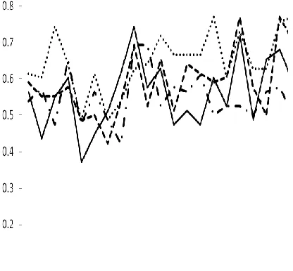
zeros varies between 40% and 80% and similar pattern could be observed in all other places.

Figure 1: Proportion for presence of zeros in the data collected at Pulicat during low tide.

Also, if the sample counts are sampling zeros, it might not be sensible to use 0.0 as the “best” estimate of a probability (Agresti, 1990), Bayesian procedure provides a more appealing way of smoothing these zeros with an appropriate prior inclusion in the analysis; following is a simple WinBUGS code for estimating proportion using a simple non-informative prior whereas Kamal et al (2011) have attempted a species specific analysis with experts‟ opinion as informative prior.

MODEL {

for ( i in 1:k) {

x[i] ~ dbin(p[i], n) #Binomial Likelihood

p[i] ~ dbeta(1, 1) #Non-informative prior for proportion U(0,1) }

}

A partial list of the entire 25 results from this analysis has been presented in Table 1. It could be observed that Bayesian procedure provides an easier as well as a better way of smoothing zeros present in the data set. Also, a range of proportion for the presence of each taxa could be estimated that vary over a tidal criterion; analysis records a proportion of as low as 0.1% to a maximum of 27.7% as an overall value. However, individual proportions for the respective taxa could be comparable in a similar way to understand the nature of presence more specifically; for example, Harpacticoids records the highest among all as 16.9% to 27.7% and Collembolans, Nermertines. Halacarids, Bivalves, Insects, Rotifers, and Cladocerans share the least value status as 0.01% to 0.02%. Further, it could be observed from Table 1 that the standard deviations (sd) associated with point estimate (mean) do not vary with alarmingly high values; and the variation would reflect in the

lower and upper limit of 95% confidence interval presented in Table 1 as 0.025 and 0.975 percentiles of MCMC output.

VI. CONCLUSION

Bayesian inference has been accepted as a more flexible and pragmatic statistical principle among ecologists for estimating parameters of interest and expressing the degree of confidence or uncertainty in those estimates (Ellison, 2004). The platform provides a better methodology to realize and work on the challenges that prevail between statistical and subject matter readers. As observed in Piegorsch et al (1998) “the resulting quantitative methodology will best represent good statistics, good science, and good public policy”.

The Bayes estimation of proportions seems to possess certain inherent properties, a better approach for estimating the summary measures that are widely used in practice. Further, irrespective of the choice of flat or informative priors, the approach of smoothing cells through Bayesian approach yield considerably valuable information about the parameter of interest, especially in a sparse data. In conclusion, the Bayes approach offers a language and tool set for studying most of the uncertainties in complicated problems, and therefore provides a better method for analyzing uncertainty in real world problems.

REFERENCES

[1] Agresti. A., (1990). Categorical Data Analysis. John Wiley & Sons, New York.

[2] Altaff, K., Naveed, M.S. and Sugumaran,J., (2004). Meiofauna of Chennai coast of Bay of Bengal with special reference to sampling and extraction methods. Convergence, 6: 61-90.

[3] Berger J (2006). The case for objective Bayesian analysis. Bayesian Analysis: 3; 385 – 402.

[4] Carlin PB and Chib S (1995).Bayesian Model Choice via Markov Chain Monte Carlo Methods. J.R. Statist. Soc. B: 57; 473 – 484.

[5] Casella G and Berger RL (2002). Statistical Inference, Duxbury, Belmont, CA.

[6] Casella G and George EI (1992). Explaining Gibbs sampler. The American Statistician: 46; 167 – 174.

[7] Chib S and Greenberg E (1995). Understanding the Metropolis-Hastings Algorithm. The American Statistician: 49; 327 – 335.

[8] Cressie, Noel, Calder, Catherine A., Clark, James S., Ver Hoef, Jay M., and Wikle Christopher K., (2009). Accounting for uncertainty in ecological analysis: the strengths and limitations of hierarchical statistical modeling Ecological Applications, 19: 553-570.

[9] Dunson, D.B., (2001). Practical advantages of Bayesian analysis of epidemiologic data. American Journal of Epidemiology, 153: 1222 – 1226. [10] Ellison, M. A., (1996). An Introduction to Bayesian Inference for

Ecological Research and Environmental Decision-Making, Ecological Applications, 6: 1036-1046.

[11] Ellison, M. A., (2004). Bayesian inference in ecology, Ecology Letters, 7: 509–520.

[12] Gelman A (1996). Inference and monitoring convergence. In: Gilks WR, Richardson S and Spiegelhalter DJ, ed. Markov Chain Monte Carlo in practice. Boca Raton, Chapman & Hall/CRC.

[13] Gelman A, Carlin JB, Stern HS and Rubin DB (1995). Bayesian Data Analysis. Chapman & Hall, London.

[14] Goldstein M (2006). Subjective Bayesian analysis: principles and practice. Bayesian Analysis: 3; 403 – 420.

[16] Higgins, R.P. & Thiel,H., Introduction to the study of Meiofauna, Smithsonian Inst. Press,(1988) 488p

[17] Hunter, J S., (1994). Environmetrics: an emerging science. In Environmental Statistics (G. P. Patil and C. R. Rao, eds) Handbook of Statistics, 12 1-7. North-Holland, Amsterdam.

[18] Kamal Nasir, V., Subbiah, M., Srinivasan, M.R., Altaff, K., and Naveed, M.S., (2011). Bayesian Estimation of Meiofaunal Population using elicited information – A study with experts‟ opinion in Ecological Models, Accepted for publication in Indian Journal of Marine Sciences.

[19] Kerman J and Gelman A (2006). Tools for Bayesian data analysis in R. Statistical Computing & Statistical Graphics; 17; 9 – 13.

[20] Martin, T G, Wintle, A W, Rhodes, J R, Kuhnert, P M, Field, S A, Low-Choy, S J, Tyre, A J and Possingham, H.P., (2005). Zero tolerance ecology: improving ecological inference by modeling the source of zero observations. Ecology letters, 8: 1235 – 1246.

[21] Piegorsch, W.W., Smith, E.P., Edwards, D. and Smith, R.L. (1998). Statistical advances in environmental science, Statistical Science. 13: 186-208.

[22] Robert CP and Casella G (2004a). Introduction to the special issue: Bayes then and now. Statistical Science: 19; 1 – 2.

[23] Robert CP and Casella G (2004b). Monte Carlo Statistical Methods. Springer, New York.

[24] Royle, J.A. and R.M. Dorazio., (2006). Hierarchical models of animal abundance and occurrence. Journal of Agricultural, Biological, and Environmental Statistics, 11: 249-263.

[25] Rubin, D. B., (1984). Bayesianly justifiable and relevant frequency calculations for the applied statistician, Annals of Statistics, 12: 1151 – 1172.

[26] Smith AFM and Roberts GO (1993). Bayesian computation via the Gibbs sampler and related Markov Chain Monte Carlo methods. J.R. Statistical Soc. B: 55; 3 – 23.

[27] Spiegelhalter, D. J., Thomas, A., Best, N. G. and Lunn, D., (2003). WinBUGS User Manual (Version 1.4). Cambridge: Mrc. Biostatistics Unit, www.mrc-bsu.cam.ac.uk/bugs/

[28] Stephens, P. A., Buskirk, S. W. and Rio, C. M., (2006). Inference in ecology and evolution, Trends in Ecology and Evolution, 22: 192 – 197.

AUTHORS

First Author – Subbiah, M ,M Sc M Phil, Ph D, L.N

Government College, Ponneri, Tamilnadu, India. [email protected]

Second Author – Kamal Nasir, V , M Sc M Phil, The New

College, Royapettah, Chennai, Tamil Nadu, India. [email protected]

Third Author – Srinivasan, M.R M Sc MBA Ph. D, University

of Madras, Chennai, Tamilnadu, India. [email protected]

Fourth Author – Naveed, MS M Sc M Phil Ph D, The New

College, Royapettah, Chennai Tamil Nadu, India. [email protected]

Correspondence Author – Subbiah, M ,M [email protected]

APPENDIX

Table1: Point and Interval estimation for the proportions of each taxa from the samples of Pulicat based on four low tide period

Taxa Low 1 Low 2 Low 3 Low 4

mean sd 0.025 0.975 mean sd 0.025 0.975 mean sd 0.025 0.975 mean sd 0.025 0.975