Application of spreadsheet and queuing network model to capacity optimization in product development

(1)

QUEING NETWORK MODEL TO CAPACITY

OPTIMIZATION IN PRODUCT

DEVELOPMENT

MUHAMMAD MARSUDI

DZURAIDAH ABDUL WAHAB

CHE HASSAN CHE HARON

WORLD CONGRESS ON SCIENCE

ENGINEERING AND TECHNOLOGY

WCSET 2009

28-30 OCTOBER 2009

(2)

Application of Spreadsheet and Queuing

Network Model to Capacity Optimization in

Product Development

Muhammad Marsudi, Dzuraidah Abdul Wahab, and Che Hassan Che Haron

Abstract— Modeling of a manufacturing system enables one to

identify the effects of key design parameters on the system performance and as a result to make correct decision. This paper proposes a manufacturing system modeling approach using a spreadsheet model based on queuing network theory, in which a static capacity planning model and stochastic queuing model are integrated. The model was used to improve the existing system utilization in relation to product design. The model incorporates few parameters such as utilization, cycle time, throughput, and batch size. The study also showed that the validity of developed model is good enough to apply and the maximum value of relative error is 10%, far below the limit value 32%. Therefore, the model developed in this study is a valuable alternative model in evaluating a manufacturing system.

Keywords—Manufacturing system, product design, spreadsheet

model, utilization.

I. INTRODUCTION

E

V E N though world has moved beyond the industrial age

and into the information age, manufacturing remains an important part of the global economy. There is a need for the pervasive use of modeling and simulation for decision support, in current and future manufacturing system, and several challenges need to be addressed by simulation community to realize this vision [ 1 ] .

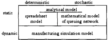
Various factors should be considered before modeling manufacturing system. They are the system complexity, degree of detail and accuracy, data and time availability, software availability, skill personnel, etc. N o single modeling tool is able to satisfy all these factors and for that reason several modeling approaches have been introduced. Generally, there are two approaches used to model manufacturing system, they are a simulation model and an analytical model [2]. As shown on Fig. 1, an application of these two models

F. A. Author is the lecturer of Poliban, Banjarmasin (Indonesia) and also the researcher at Tun Hussein Onn University of Malaysia 86400 Parit Raja, Johor Darul Takzim - Malaysia (phone: 6074537771; fax: 6074536080; e¬ mail: marsudi® uthm.edu.my).

S. B. Author, is the lecturer of Faculty of Engineering at National University of Malaysia, 46000 UKM Bangi, Selangor Darul Ehsan - Malaysia (e-mail: [email protected]).

T. C. Author is the lecturer of Faculty of Engineering at National University of Malaysia, 46000 UKM Bangi, Selangor Darul Ehsan - Malaysia (e-mail: [email protected]).

can be differentiated based on data randomness time dependency. The data randomness can be categorized into two models i.e. deterministic and stochastic. On the other hand for the time dependency it is also categorized as static models and dynamic models. The dynamic models are simulation models including deterministic models and stochastic models, and the static models are analytical model and queuing network model.

There are performance measures on manufacturing system commonly estimated by modeling and simulation. They are throughput, time in system for parts, parts spend in queues, queue size, timelines of deliveries, and capacity utilization of equipment [3]. Although there were many studies [4, 5, 6] by previous researchers that related to capacity analysis in product development, this topic is still open and necessary to be studied. This paper discusses the performance measures of capacity utilization related to product development. The objective of this study was also to describe a mathematical model which is a result of combination between a spreadsheet and a complex queuing network model. The complex queuing network means a manufacturing system having multi-stage production line to produce product assembly. The mathematical model used in this study also considers a few parameters such as utilization, cycle time, throughput, batch size, and reliability factor. This reliability factor consists of normal yield, reduced yield and scrap yield parameters at a certain workstation. The product assembly in automotion industry was focused in this study.

deterministic stochastic

dynamic

analytical model spreadsheet

model

mathematical model of queuing network

[image:2.595.324.512.565.634.2]

manufacturing simulation model

Fig. 1 Different modeling tools to model manufacturing system

II. RELATED WORK

(3)

installed, used, serviced, and retired or recycled. Ignoring downstream issues leads to poor product design that may cause unforeseen problems and excessive costs downstream

[21-Unfortunately, downstream life cycle is difficult to predict accurately during the early design phases. To overcome this problem, many researchers [3, 4, 5, 6, 7] have presented the results of their study using a certain approach during product design. For example, Koo et al. [3], Taylor et al. [4], Bermon

et al. [5], Soundar and Bao [6] used a mathematical model to

analyze capacity related to product development. Shady et al.

[7] who had presented the application of a spreadsheet model to simulate the layout of electrical power transmission project in USA. However, these studies do not address the application in multi-stage production lines which are the current trend in modern production lines.

Taylor et al. [4] used a capacity analysis model to

determine the maximum product quantity at electronic assembling facilities. The analysis is conducted on existing products mixed with the detail design of new product. In case where maximum production quantity is not enough, the design of the new product should be changed in order to avoid production process at critical or bottleneck resources. By taking this action, production quantity will be increased to an acceptable level. However, this capacity analysis model does not consider the manufacturing cycle time of the system.

Bermon et al. [5] have studied a capacity analysis model at

a production line producing various products. The approach made was focused not only on product design but also to have a decision support that enables quick analysis. They defined available capacity as the number of operations that can accomplished by the equipment in a day. The information about available equipments, products, and required operation are known, the equipment capacities that conform to both required throughput and existing limitations are allocated. Cycle time data and capacity are located at a level below the existing available capacity. The differences between the existing capacity and allocated capacity are referred as contingency factor. A good contingency factor will prevent the queuing time average of equipment groups from exceeding the processing time determined before. The queuing model approach was used to model the relationship between utilization and queuing time. By using this approach, they can verify the capacity of manufacturing system in terms of capability to achieve the required throughput for a reasonable

manufacturing cycle time. Although the study by Bermon et

al. [5] is valuable, they did not discuss product development

activities.

A few researchers described capacity planning approaches as a part of planning and control systems of traditional manufacturing [9, 10]. These approaches identify how many times, when, what type, and where manufacturing system should increase its capacity in order to obtain the required throughput. Therefore its general objective is to minimize equipment cost, inventory, and cycle time. There are many other models that are not very significant and also less accurate. Furthermore, these models do not include

applications for multi-stage manufacturing system.

Soundar and Bao [6] presented a planning that relates product design effects to manufacturing system. They suggested the use of mathematical models and simulation to predict various performance parameters including manufacturing cycle time. However, the approach was very general and no examples were discussed in their paper.

Johnson and Montgomery as stated in Aomar [11] presented a mathematical formulation for the product-mix problem as a constrained Linear Programming (LP) model. They found that many firms have benefited from the use of this LP model especially in making product-mix decision. In order to apply the LP model, many input data from the industry are required such as the minimum production level of each product type in the planning period, number of units in each resource that are required to produce one unit of each product, and the amount of each resource available during the planning period. Their study did not discuss product development and also no example given for showing the application of their theory.

Walid Abdul Kader [12] presented a study on certain parameters of modern production lines having a variety of product processes in a batch production environment, which is in relation to capacity estimation. These parameters include the set-up time, the product mix, and the reliability of the stations composing the systems. However, it will be complicated and needs more calculation whenever the manufacturing system has more than two stage production line.

Chincholkar et al. [13] presented an analytical model for

estimating the total manufacturing cycle time and throughput of the manufacturing system. The development of this model follows the standard decomposition approach for queuing network approximations [14]. Their goal was to analyze these facilities quickly by avoiding the effort and time needed to create and run simulation models. They present numerical results that show how the queuing network model yields results similar to those of a simulation model. However, these studies do not address the application in a multi-stage process which is very important for this study.

Wei and Thornton [15] have analyzed the production system performance evaluation of Boeing's aircraft tube manufacturing plant by using complex queuing network. Herrmann and Chincholkar [16] used the same complex queuing network like Wei and Thornton did to analyze PCB (printed circuit boards) production line in electronic industry.

III. MATHEMATICAL MODELING

Queuing models can represent a wide variety of manufacturing systems. Often, the model is a network of queues, where each node represents a different manufacturing resource or workstation. The information about the probability distributions of j o b arrivals and j o b processing times at each node, one can determine the average time in system for a j o b .

(4)

used in the spreadsheet model based on the queuing network are described. This queuing network is the same as Wei and Thornton [15] used but the original algorithms is modified by considering reliability factors at each work station for processing a certain product. These reliability factors are normal yield, scrap yield, and reduced yield. Therefore for processing product i at station j , the normal yield, scrap yield,

and reduced yield is symbolized a s v, " , V * , and y^

respectively.

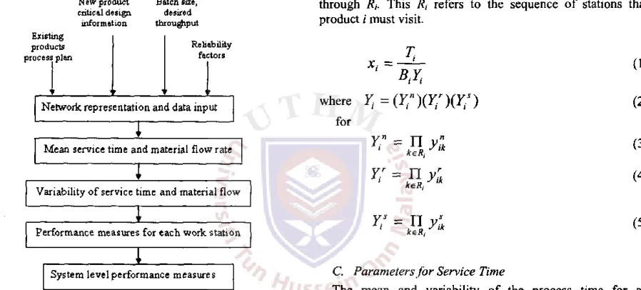
The proposed spreadsheet model in this paper has the fundamental procedure for evaluating performance measures and it is shown in Fig. 2. The procedure is adapted from the model developed by Koo et al. [3] although a few adaptation needed.

New product critical design information

Batch size, desired throughput Existing

products process plan

Reliability factors

Network representation and data input

T

Mean service time and material flow rate

Variability of service time and material flow

Performance measures for each work station

[image:4.595.78.527.275.478.2]

System level performance measures

Fig. 2 Procedure to calculate performance measures on spreadsheet model

A. Input and Data Notation

The input data and notations used are listed below.

BT - j o b size of product i at release

Cy - S C V {squared coefficient of variation) of the set up time

c'y - SCV of the part process time

C,r - SCV of j o b interarrival times for product i

cdj - SCV of interdeparture times at station j

Ttij - mean time to failure for a resource at station j

mrj - mean time to repair for a resource at station j

rij - the number of resources at station j

Sy - mean j o b setup time of product /' at station j

Tj - desired throughput of product i (parts per hour) ty - mean part process time of product /' at station j

y"j - normal yield of product i at station j yfj - reduced yield of product i at station j yt - scrap yield of product /' at station j

Both stj and ttJ are based on the design parameters of

product i.

B. Parameters for Material Flow

Release rate Release rate of product i (jobs per hour) x,

includes three parameters. These parameters are desired

throughput, j o b size, and cumulative yield of product i (Y,)

through Rj. This Rt refers to the sequence of stations that

product i must visit.

(1)

(2)

BY,

where ^ = ( ^ ) ( ^ ) ( ^ )

for

k<=R.

(3)

(4)

(5)

C. Parameters for Service Time

The mean and variability of the process time for an individual product are given as the parameters of input data. However, there are many factors that affect this process time and therefore the adjustment of process time of a product i at a

workstation j should be done. For example, these factors are

product mix, batch size, setup time, and design parameters of product.

Mean part process time of product i at station j is

differentiated based on the type of station. These types are categorized into work station and inspection station. If a station is a work station, the adjusted process time is given in formula (6). On the other hand, the formula (7) is for an inspection station.

(6)

(7)

Another parameters for service time are aggregate process

(5)

t = (8)

(9)

In this case Vj is the set of products that visit station j , and

Aj is availability of a resource at station j which is

formulated as:

m.

(10)

D. Approximation of Performance Measures

Given all parameters described in the previous sections, static performance such as resource utilization can be calculated. The resource utilization is one of the performance measures commonly used in manufacturing systems. Sometimes, it is the most important factor for decision making, especially when a large capital investment is needed.

The average resource utilization at station j ( m . ) is:

Uj = — Z x , (11)

Other than static performance above, we can also calculate stochastic performance which is cycle time parameter. The

average cycle time at station j ( CT*), and the average cycle

time of j o b s of product i (CT,) are formulated as follows:

" y d - " , )

(12)

(13)

CT.'TCT]

JeR,

where c", is SCV of interarrival times at station /, and c* is

j J j

SCV of the modified aggregate process time:

° — d

Cj ~ Cj-i • 2 < ; < y

m ,

:'

J

=c+

J+

2A

J

(l-A

J

)

1

f

(14)

(15)

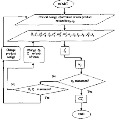
Referring to the above discussion, Fig. 3 is the flow chart as a guidance to improve the resource utilization:

START ")

Critical design information of new product related to Sj,

I

.S" Bl.T,,c'rc^.df,c,).mj.m'l.nj.sf,tf.yt,y"f.yl

I

Change Change fy, product

T, or both design j of them

^fzzzr

Bp Tt maximum?

Uj rnaximum? "'--^

CT,

_J !

[image:5.594.319.508.107.303.2]

( END )

Fig. 3 The framework for improving resource utilization

IV. IMPLEMENTATION M O D E L

The spreadsheet model here is constructed using Microsoft Excel. T o implement the proposed model on the spreadsheet, a spreadsheet program should be configured so that both its data structure and its computational methodology conform to spreadsheet characteristics. The spreadsheet program proposed consists of three main parts which are input block, intermediate result block, and output block. Another part is graph section which is related directly to output block. The function of the graph section is to show output results from output block as graph performance.

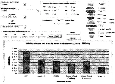
All the calculation procedures and formulae described in the previous section will be encoded to the intermediate result block and output block. On the other hand, all data required for modeling a system are entered in the input block. Clearly, once the data are entered in the input block, intermediate calculations are performed before finding final performance measures displayed on the output block. These calculations are carried out in the intermediate result block. Intermediate calculations include parameters such as the mean and variability of interarrival time and service time for p r o d u c t ; at each workstation. Fig. 4 and 5 show spreadsheet model for input block and output block - graph section, respectively.

. F R O N T D O O R L H / R K P R O T O N W I R A

.

v~ RF 1.01 LINES

B3H

!t3

1 4

$***+

[image:5.594.313.525.590.687.2]

(6)

us.

[image:6.595.80.271.105.245.2]

VttMtn&Wn m WMfewttittlMI fi.**ie N t S H t

Fig.5 The spreadsheet for Output Block - Graph section

V. M O D E L V A L I D A T I O N

A validation was performed by comparing the output of the spreadsheet model with those obtained through an existing simulation model i.e. Arena® software. In this case, quantity and type of data to be entered to the spreadsheet model are the same with the quantity and type of data to be entered to

A r e n a0 model. The output was compared with parameter

utilization and manufacturing cycle time. The performance of

A r e n a6 model user interface in this study is shown in Fig. 6.

For this purpose, a local automotive car parts manufacturing company was utilized. The production line consists of many workstations as shown in Fig. 7, and type of product to be processed in this line is front door-sash as shown in Fig. 8. There are twelve workstations, each of which is responsible for saw cutting, oil press cutting, plasma welding (surface),

knocking, plasma welding (back), welding C 02, manual

welding, die matching, finishing (single), finishing (double), checking, and anti-rust oil spray.

The experiments were carried out for two different cases. The first case was for 82 u n i t ^ a t c h (batch size) and 29 units/hours (throughput), and the second case was for 82 unuVbatch and 35 units/hours. For the first and the second case, utilization and manufacturing cycle time parameters between two models i.e. spreadsheet model and simulation model, w a s compared. T h e comparison described in Table I and Table III for utilization, Table II and Table IV for manufacturing cycle time parameter.

Saw cutting

Oil press cutting

Plasma welding (surface)

Knocking

Finishing (single)

Die matching

Manual welding

Welding

C02

U

Plasma welding (back)

Finishing (double)

Checking Anti-rust

oil spray Finished product

Fig.7 A schematic of workstations in an assembling production Line

Table I and Table II show that the average relative error of spreadsheet results is 6% and 7 % for utilization and manufacturing cycle time parameters respectively. This relative error value is far below 3 2 % which is the limit value determined by Koo et. al [3]. In Table III and Table IV, the average relative error is 6 % and 1 0 % for utilization and manufacturing cycle time, respectively. Based on this data, the spreadsheet model developed has shown its validity for being applied.

Inner B-Pillar Olass guide

Glass guide

[image:6.595.314.521.117.234.2]

Inner B-Piilar

Fig. 8 Front door-sash for car

TABLE I

UT I L I Z A T I O N A T E A C H W O R K S T A T I O N F O R I N P U T 8 2 U N I T S / B A T C H A N D

2 9 U N I T S / H O U R

Workstation Spreadsheet _model Simulation

model Relative error

Saw cutting 0.7992 0.8736 -0.09

OP cutting 0.0905 0.0994 -0.09

PL welding (surf.) 0.7778 0.8534 -0.09

Knocking 0.0741 0.0810 -0.05

PL welding (back) 0.5398 0.5885 -0.09 Welding C 0 2 0.9798 0.9058 0.08 Manual welding 0.2805 0.2560 0.10

Die matching 0.1848 0.1689 0.09

Finishing (single) 0.6835 0.6181 0.10 Finishing (double) 0.6611 0.5920 0.11

Checking 0.0658 0.0445 0.48

[image:6.595.209.523.345.682.2]

Anti rust oil spray 0.7908 0.6781 0.17 Average relative error 0.06

[image:6.595.64.270.572.692.2]

(7)

TABLE II

M A N U F A C T U R I N G C Y C L E T I M E (SECONDS) A T E A C H W O R K S T A T I O N FOR INPUT

82 U N I T S / B A T C H A N D 29 U N I T S / H O U R

Saw cutting 2131.7 2170.8 -0.02

OP cutting 232.1 248.0 -0.06

PL welding (surf.) 1994.8 2121.6 -0.06

Knocking 190.1 202.2 -0.06

PL welding (back) 1384.5 1465.8 -0.06

Welding C02 2512.8 2231.3 0.13

Manual welding 719.4 638.8 0.13

Die matching 474.0 420.9 0.13

Checking 145.5 111.3 0.31

TABLE III

U T I L I Z A T I O N A T EACH W O R K S T A T I O N FOR I N P U T 82 U N I T S / B A T C H A N D

35 U N I T S / H O U R

Saw cutting 0.7922 0.9000 -0.12

OP cutting 0.0905 0.1027 -0.12

PL welding (surf.) 0.7777 0.8789 -0.12

Knocking 0.0741 0.0835 -0.11

PL welding (back) 0.5396 0.6059 -0.11

Welding C02 0.9797 0.9092 0.08

Manual welding 0.2805 0.2562 0.09 Die matching 0.1848 0.1688 0.09 Finishing (single) 0.6835 0.6146 0.11 Finishing (double) 0.6611 0.5866 0.13

Checking 0.0658 0.0438 0.50

TABLE IV

M A N U F A C T U R I N G C Y C L E T I M E (SECONDS) A T E A C H W O R K S T A T I O N FOR INPUT

82 U N I T S / B A T C H A N D 35 U N I T S / H O U R

Saw cutting 2031.7 2157.0 -0.06

OP cutting 232.1 246.4 -0.06

PL welding (surf.) 1994.8 2102.2 -0.05

Knocking 190.1 200.3 -0.05

PL welding (back) 1384.5 1448.3 -0.04

Welding C02 2512.8 2148.0 0.17

Manual welding 719.4 615.0 0.17

Die matching 474.0 405.2 0.17

Checking 145.4 105.0 0.38

VI. C O N C L U S I O N

Spreadsheet model discussed in this paper try to integrate

deterministic-static feature and stochastic feature. This spreadsheet model enables the designer to m a k e various

changes in decision parameters (i.e. sy and ty are affected b y design parameters) and examine the effect of the changes on

performance measures very easily and quickly. In other words, the time needed for design phase can be reduced for a

new product because redesign activities have been done in the

earlier stage of design phase. In other words, design changes initiated as a result of analysis using the model are possible to

b e performed in the earlier stage of design phase of a product. So the time for launching n e w product can also be reduced.

The study also showed that the validity of spreadsheet model is good enough to apply and m a x i m u m value of relative error

is 10%, far below the limit value suggested by Koo et al. [3]. Besides the use of A r e n a " software for validation process of

the spreadsheet model, future study can b e directed to the use of another existing simulation tool such as W i t n e s s0 software.

ACKNOWLEDGMENT

T h e authors would like to thank the Ministry of Higher Education, Malaysia for supporting this research under the

Fundamental Research Grant Scheme (FRGS).

Re f e r e n c e s

[I] Fowler, John, W., and Rose, O., "Grand challenges in modeling and simulation of complex manufacturing system", Simulation, Vol. 80, No. 9, pp. 469-476, 2004

[2] Cooper, R.G., "Third - Generation new product process", Journal of

Product Innovation Management, Vol. 11, No. 1, pp. 3-14, 1994

[3] Koo, P.H., Moodie, C.L., and Talavage, J.J., "A spreadsheet model approach for integrating static capacity planning and stochastic queuing models", International Journal of Production Research, Vol. 33, No. 5, pp. 1369-1385, 1995

[4] Law, A.M., and McComas, M.G., " Simulation of manufacturing system", Proceedings of the Winter Simulation Conference, pp.56-59, 1998

[5] Taylor, D.G., English, J.R., and Graves, R.J., "Designing new products: Compatibility with existing product facilities and anticipated product mix", Integrated Manufacturing Systems, Vol. 5, No. (4/5), pp. 13-21, 1994

[6] Bermon, S., Feigen, G., and Hood, S., "Capacity analysis of complex manufacturing facilities", Proceedings of 34* Conference on Decision &

Control, New Orleans, December 1995.

[7] Soundar, P., Han, P.B., "Concurrent design of products for manufacturing system performance", Proceedings IEEE International

Engineering Management Conference. Ohio, Dayton. 1994

[8] Shady, R., Spake, G., and Armstrong, B., "Simulation of a new product work cell", Proceedings of Winter Simulation Conference, USA. 1997 [9] Hopp, W.J., Mark, L.S., "Factory Physics", Irwin/McGraw Hill, Boston.

1996

[10] Vollmann, T.E., Berry, W.L., and Whybark, D.C., "Manufacturing planning and control systems", 4th edition., Irwin/McGraw-Hill, New York, 1997

[II] Aomar, R., "Product-mix analysis with discrete event simulation",

Proceedings 2000 Winter Simulation Conference, USA. 2000.

[12] Walid Abdul Kader, "Capacity improvement of an unreliable production line - An analytical approach", Computer & Operations Research, No. 33, pp. 1695-1712, 2008

[13] Chincholkar, M.M., Burroughs, T., and Herrmann, J.W., "Estimating manufacturing cycle time and throughput in flow shops with process drift and inspection", Institutes of Systems Research and Department of

Mechanical Engineering University of Maryland.lOM

[14] Papadopoulos, H.T., Heavey, C , and Browne, J. "Queuing theory in manufacturing systems analysis and design ", Chapman and Hall, London, 1993

[15] Yu-Feng,W. and Thornton, A.C., "Concurrent design for optimal production performance", Paper DETC2002/DFM-34163 in CD-ROM

Proceedings of 2002 ASME Design Engineering Technical Conference,

Montreal, Canada. 2002.

[16] Herrmann, J.W., and Chincholkar, M., "Design for Production: A Tool for reducing manufacturing cycle Time", Paper DETC2000/DFM-14002