Combined Methods for Solving the Variational Problems of a Special Type

Combined Methods for Solving the Variational

Problems of a Special Type

Valery I. Struchenkov

Moscow State University of Radio Engineering, Electronics and Automation,Moscow, Russia *Corresponding Author: [email protected]

Copyright © 2014 Horizon Research Publishing All rights reserved.

Abstract

Under study is the problem of searching the extremal of given functional ( two or three-dimensional curve ), which must satisfy a number of predetermined restrictions. A specific feature of the desired curve is that it should consist of elements of special types, whose parameters are limited. The number of elements is unknown and should be determined in the process of solving the problem. Such problems arise in particular in designing linear structures routes. In the case searching of two-dimensional extremal piecewise linear and piecewise parabolic curves are considered. Such problems arise in the design of optimal longitudinal profile of railways and roads. Multi-stage approach is proposed using the methods of nonlinear and dynamic programming. At the first stage we define broken line consisting of elements of small length, using nonlinear programming. At the second stage we determine a number of the elements and the initial approximation, using dynamic programming. At the third stage we find the optimal decision using a special non-linear programming algorithm.

Keywords

Functional, Extremal, Objective Function, Nonlinear Programming, Dynamic Programming, Reduced Antigradient

1. Introduction

Many of optimization problems from different practice areas are reduced to finding two or three dimensional curves, which must satisfy the conditions of smoothness and other restrictions. Moreover some integral index which uniquely defined for each admissible curve must take minimum. In other words, we want to find the extremal of the given functional, satisfying the system of restrictions.

Examples of such tasks can serve as the search of optimal routes (plan and the longitudinal profile) proposed roads and other linear structures, both at the stage of new construction and reconstruction phase. The functional reflects construction costs or reduced expenditures on construction and operation of road.

The principal feature of these problems is that the desired curve (extremal) should consist of elements of a given types. Depending on the type of structures as elements can be used straight-line segments, arcs circles, parabolas, clothoids, etc. Element parameters must satisfy the restrictions on the first derivatives and curvature. The element lengths are also limited. The number of elements of projected curve is unknown.

Expediency of optimization projects of such expensive facilities like railways and roads is obvious. In particular in the conditions of rugged relief and complex geology the cost of construction and subsequent operation can be significantly reduced at the optimum location of the projected route of the road on the ground. It was established in the operation of the first CAD, in which the design of the longitudinal profile of new railways was carried out with the use of optimization program [ 1 ].

Marked features of the problem hampering the development of algorithms and programs as well as the lack of interest of designers and builders to reduce construction costs, have led to the fact that the mathematical methods of optimization runs are not practically used. Considered sufficient to use different kinds of heuristic algorithms in the process of interactive design.

Currently, even in the most developed modern systems of automated design (CAD), such as CARD-1 [2]. Bentley Rail Track [3], or their Russian analogy Topomatic Robur [4] and Geonics [5] computer is used to solve related routine tasks, but not as a tool to develop optimal design decisions. It is known that in the same conditions, having the same information, different specialists offer a variety of design solutions. Consideration of a limited number of options intuitively appointed does not guarantees closeness to the optimum final result of this process. At the same time it is known that relatively small changes in the route position on the ground can cause significant changes in the cost of construction and maintenance [6].

Consequently, the problem of developing adequate mathematical models and mathematically correct algorithms optimize routes of new roads remains relevant. This is the main way of improving CAD of linear structures.

variational problem which is not solved by classical methods can be solved using a combination of methods of nonlinear and dynamic programming.

This article gives a general statement of the original variational problem and considered the most typical special cases. The following are the mathematical models. The case of two-dimensional search curve considered in detail, starting with the identification number of elements and ending with the optimization of their parameters. The realization of the methods of nonlinear and dynamic programming in concrete algorithms will be based on the specifics of the system of restrictions.

The aim of the study was to develop a mathematical model, methods and algorithms for solving variational problems which have important features, to improve CAD linear structures by using computer for optimization of their routes.

2. Mathematical Model

The task is as follows: find a three-dimensional curve x (s), y (s), z (s), for which achieved

(1)

Here s-current and S-unknown total length of the curve connecting two given points A and B. F (x (s), y (s), z (s)) - given function with continuous first partial derivatives with respect to all three their arguments. Function F can contain as arguments the partial derivatives of x (s), y (s), z (s),which are constrained. Inequalities constraints can be imposed on the coordinates of the individual points of the required curve. For optimal linear structures routing x (s), y (s) - set up of the plan of the route, and z (s) - its longitudinal profile. In this case z (s)-single - valued function, and

dz v

ds

≤

,where ν (maximum longitudinal slope ) has a value of a few parts per thousand , and so difference between the length of the desired curve and the length of its projection on the horizontal plane is almost immaterial. Restriction on the slope may be bilateral. Limited not only the first derivative in the longitudinal profile, but also the curvature in plan and longitudinal profile, as well as the coordinates of individual points (for example, when crossing watersources and existing communications).

The problem has significant differences from the problems considered in the calculus of variations [7]. First of all is the presence of inequality restrictions. Even in the absence of additional conditions under which the desired curve should consist of elements of a given types, these features do not allow the use of the apparatus of the classical calculus of variations, in particular Euler equations [7], to solve the problem.

If in (1) the functions x (s), y (s) are given, then we get the

problem of finding a flat curve z (s), with z (s) - single-valued function.

Another particular problem arises when we are looking for a curve in the plane X Y i.e. functions x (s), y (s). In this case, the desired curve is not necessarily a single-valued function . For line structures routing search z (s) - corresponds to the optimal design of the longitudinal profile for a given variant of the route plan. This problem can be independent when we routing in populated areas due to lack of opportunities in variation of the route plan. Search plane curve x (s), y (s) corresponds to the design route plan in circumstances where the longitudinal profile is uniquely determined by the plan or weakly depends on it. An example is the trenching at a given depth, the routing of new railway in strenuous conditions [8], or the design of the reconstructed railway route plan (spot surfacing of a track).[8].

Let us consider some two-dimensional problems for railways routing. If we design the longitudinal profile the desired line z's) - is a broken line connecting the start and end points, the number of its elements is unknown.

If we denote the ground profile H (s) then in the first approximation the problem is as follows. For given H (s) find such a broken z (s), which satisfies all the constraints, and gives

(2)

where S0- known length of the plan, and function F corresponds to cost of construction for elementary length.

Realistic models must take into account the design of transverse sections of subgrade, the presence of culverts and other man-made structures, the distribution of earth masses and production methods of excavation, etc. These models are discussed in detail in [8, 9, 10].

Knowing the number and lengths of required elements of the broken line we can analytically express all restrictions on z (s), if we take as unknowns zi (i = 1, 2, ..., n) i.e. ordinates of its nodes. These restrictions are divided into three groups.

1. On ordinates at individual points

z

i

≤

z

imax

or

z

i

≥

z

imin

.

2.On slopes of all elements

a

i

≤

(z

i+1

-z

i

)/s

i

≤

b

i

(i=1,2,…,n-1)

Here si - length elements. These limits are discrete analogs of restrictions on the first derivative.

3. On differences of the slopes adjacent elements:

c

i

≤

(z

i+2

-z

i+1

)/s

i+1

-(z

i+1

-z

i

)/s

i

≤

d

i

These limits are discrete analogues restrictions on the curvature.

In view of the smallness of the slope the length of the element and its projection practically coincide.

Integral (2) becomes the sum [9,10] and we obtain the following nonlinear programming problem with linear constraints system. Find minФ (x, c) with Ax≤b , where x-vector of unknowns, c - vector of parameters, the matrix A and vector b - form a system of linear reartictions.Ф (x, c) - the objective function.

In the case of designing the plan of the route of different linear structures, i.e. when searching functions x (s), y (s), the required elements of the line can be straight-line segments, circles, parabolas, clothoids etc. A number of elements is unknown. Minimum length of the elements, the maximum curvature and the coordinates of individual points are given. The desired curve may be represented approximately as a broken line with more then required but known number of nodes. As variables can be taken coordinates of unknown nodes of the desired line. All restrictions can be expressed analytically through these variables. Again we have the problem of nonlinear programming, but with the nonlinear system of restrictions. When designing the reconstruction of railway tracks as variables are not convenient to take the coordinates xi, yi of

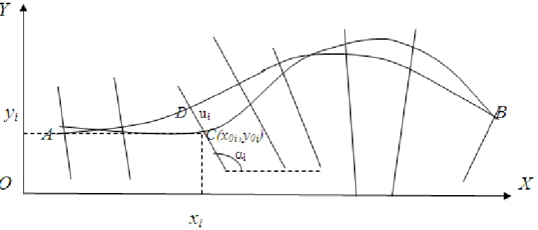
unknown nodes. Instead of this we use displacements ui along the normals at the points of the existing route plan (CD in Figure 1).

Through these displacements we can also express all restrictions on required curve. Thus we obtain the problem of nonlinear programming with fewer variables.

We obtain the following formulas for the corresponding restrictions:

1. Curvature of the circle drawn through any three adjacent points of the route plane must be within predetermined limits i.e.

kmini ≤k(ui-1,ui, ui+1) ≤ kmaxi.

This limitation of the variables are expressed as follows :

(3)

The numerator in (3) is a determinant of the third order, which includes the Cartesian coordinates of three adjacent nodes, and the denominator - the product of the distances between these points. Determinant - it doubles the area of the triangle with vertices at these points. It is well-known formula for the radius of the circle R = abc / (4S), where a, b, c are the lengths of the sides, S- area of a triangle.

At first we express the Cartesian coordinates of the intersections the normales with the route plan through the variables ui (i = 1,2, ..., n).

xi =x0i +uicos αi; yi =y0i +uisin αi

[image:3.595.111.504.557.725.2]

Then we calculate the distance between points and curvature through these coordinates. Here x0i, y0i - coordinates of the starting point on the i-th normal, αi - angle of this normal with the axis X.

2. Restrictions on the coordinates of individual points, including the conditions of intersection other communications and watercourses are recorded simply:

ck ≤ uk ≤ dk. Here k is the number of that normal which corresponds to communication or watercourse . These restrictions may be many. For a strictly fixed points ck = dk.

Restrictions on the route plan essentially nonlinear.

Nonlinear programming problems, which we obtain using the discrete representation of the desired extremal, have significant features due to the specifics of the objects. These features relate primarily to the system of restrictions on the desired extremal.

3. Features Emerging Problems of

Nonlinear Programming and Their

Solutions

None of the restrictions does not contain more than three adjacent variables. This means that in the linear case (the design of the longitudinal profile) matrix of restrictions has the block character. Blocks corresponding to the three types ,restrictions mentioned above, contain in each line only one, two or three non-zero elements. This allows us to construct an iterative process at each step of which for any set of active constraints descent direction is determined without solving systems of linear equations. As such direction we use reduced antigradient [11, 12].

If Ak -matrix of the system of active restrictions at the k-th

iteration and N(Ak)- its null space [12], the above properties

of restrictions for any active set make it easy to construct a basis in N(Ak) [13]. If C-basis matrix and f- antigradient of

the objective function, then CCT_{f, called reduced}

antigradient, is the direction of descent. Indeed, its scalar product on antigradient is nonnegative since (CCT_f,f)=(CT_f,CT_f)≥0.

The system of nonlinear restrictions, obtained at a discrete representation of route plan, in each of the inequalities contains no more than three adjacent variables. After its linearization in the current iteration point we obtain a system of linear inequalities, which has distinguished features. This allows to construct a basis of zero-space corresponding to the tangent plane. The descent from the current iteration point advantageously carry out not in the tangent plane, but along the curve in the boundary surface without disturbing the active nonlinear constraints. Tangent to the curve coincides with the direction of descent in the tangent plane. This is the meaning of the method of basic displacements [14].

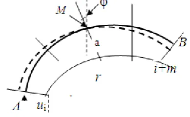
Suppose at some iteration some points with numbers from i-th to (i + m)-th lie on the curve of the maximum radius (Fig. 2). Its initial position is AB. Need to find such changes for variables

u

i

, u

i+1

, …, u

i+m

,

at which the radius remains the limit. This means that the circumference is shifted as a whole, and its any displacement can be represented as a combination of two offsets, for example, shift along a straight and rotation in a plane around a center. As the line

for shift we can take any normal with number i ≤ k ≤ i + m, as

well as the center of rotation to take the intersection of the route plan and selected normal. On Fig. 2 a point M lie on the normal with number r. Let a - amount of displacement along

the normal r , and φ-angle of rotation. If the values of a and φ

are known, the increments

∆u

k

(i ≤ k ≤ i+m

)

are calculated

by a, φ, angles of the normals with OX and baseline values

u

k

(i ≤ k ≤ i+m).

If there is one point on the circle whose

[image:4.595.333.528.238.358.2]

coordinate uj is of minimal or maximum value, then it should be taken as the center of rotation, and the corresponding j-th normal as line for shear. In this case, a = 0, and all values of the desired displacements are determined by the rotation angle.

Figure 2. Example Basic Displacement (shift + rotation).

If on the circle of maximum radius there are two or more fixed points then the desired displacement or changes of

coordinates Δuk (i ≤ k ≤ i + m) are zero.

Set of linearly independent basis displacements is an analog of basis for linear case. When linearization basis displacements we obtain basis in the corresponding zero-space.

It is important to note that these features of the system restrictions allow us to carry out modification of the active set as in the linear and nonlinear cases without cumbersome calculations . [13]

For further use of these features of the system of constraints in specific algorithms of nonlinear programming is necessary to determine the number of elements unknown extremal and to construct the initial approximation.

4. Determining the Number of Elements

and Construction of the Initial

Approximation

restrictions on the minimum length of the element. Therefore the deviation from the desired sequence elements are much smaller than the width of the source area of finding the optimal solution [14]. This allows to use previously developed algorithms of dynamic programming for solving emerging problems of approximation broken line by plane curve consisting of the elements of a given form in the presence of restrictions discussed above [15,16].

Characteristically, the limitations in this case contribute to reducing the computation time due to the reduction of the number of valid choices.

When designing the longitudinal profile of railways broken line consisting of short elements, is converted to another broken line, but with elements of a length not less than a predetermined value. Conversion algorithm discussed in detail in [8,15].

When designing the longitudinal profile of highways transformation can be carried out in the second degree parabola (in particular of the segment lines) or in circular curves with or without direct inserts. Corresponding dynamic programming algorithms are given in [8,16,17].

There are no particular difficulties in transformation of a broken line into sequence of circular curves with straight inserts when designing a route plan. Only feature is that the desired extremal in general is not an unambiguous function. Therefore, to use dynamic programming we must build the grid using normals [14] but not vertical lines. Converting of broken line into a sequence direct, clothoid, circular, clothoid , direct etc required the development of a new algorithm, because using dynamic programming for solving this problem was failed.

5. Optimization of the Initial

Approximation

Extremal obtained after converting the broken line should be considered as an initial approximation to find a final solution.

The meaning of the considered first two phases (calculation broken line and its transformation) is to find the dimension of the problem (number of elements) and to obtain the initial approximation. The matter is not in that the dynamic programming does not provide solution accuracy due to discrete variation, but in such problems as the design of the longitudinal profile of new roads, there is additional relationship of elements in cuts and fills, constructed together. The objective function in this case can not be calculated separately for each element that does not allow to use dynamic programming [14].

If desired extremal consists only of linear elements, as is the case in the designing of the longitudinal profile of the railways, the optimization of the initial approximation is carried out using the same algorithm of nonlinear programming, as at the first stage in calculation of broken line. In this case, the ordinate of any point desired extremal linearly depends on the ordinates of end points of the

relevant element. So in new algorithm was added only conversion of derivatives of the objective function with respect t nodes ordinates of initial broken line into derivatives with respect to nodes ordinates of required extremal.

When using parabolic elements in both the design of roads is convenient to take as unknowns the slopes at the end points all elements instead of their ordinates.

Consider the case of fixed slopes at the start and end points of the profile.

Equation of any parabola in Cartesian coordinates (l, H), placed at the beginning of the element has the form: H=al2 _{+bl +c, where c -ordinate of the starting point of the} element , b-slope at the starting point of the element, l - distance from the starting point of the element.

If we take as unknown slopes i.e. parameters bj (j = 1,2, ..., n +1), where n-number of elements, then through these slopes can be found the ordinate of any point , assuming that ordinate of starting point is predetermined. Indeed, the parameter

a

_j of each parabola is calculated through slopes in its start and end points, because Lj - the element length is known.

aj= (bj+1 - bj)/(2 Lj). (4) cj+1=(bj+1 + bj) Lj /2 + cj ₍₅₎ This means that for any combination of parameters bj we can calculate all the ordinates, once considered as independent variables, and, consequently, partial derivatives (gradient) of the objective function. We need to calculate consistently the parameters aj and c j +1 by the formulas (4) and (5).

Restrictions on the slopes can be written quite simply: bmin

j ≤ bj≤ bmaxj Restrictions on radii:

Lj/Rjmin1_{≤ bj+1 - bj≤ Lj/Rj}min2_.

Here Rjmin1 _{<0 and Rj}min2_{> 0 the minimum allowable radius} of convex and concave curve, respectively.

System of constraints is extremely easy, so for any set of active constraints and the slopes and radii it is possible only two options:

1. Shift in space of slopes is impossible (zero section) with the presence of at least one limited slope in the relevant section ;

2. All components of a single basis vector is equal to one (shift section), if only restrictions on radii are active. Note that in the original coordinate space zero section corresponds to a shift along the ordinate and shift section corresponds to a rotation with center at the starting point of the section.

Two ways to overcome the difficulties was proposed [14]: 1. Using the penalty function for violating restrictions on the ordinates;

2. Constructing the descent direction by solving the auxiliary systems of linear equations which number is equal to the number of active constraints on the ordinates.

Let's consider a simple way of constructing the descent direction with a special reception basis transformation. To do this, we take the canonical basis in the space of the slopes for the extremal in general. The identity matrix E corresponds to this basis .

If from k-th to k + m slope we have a zero section then the columns with the k-th to the k + m are deleted from the matrix. So zero rows are formed in the matrix .

If from r-th to r + p slopes we have a shift section then the respective columns are replaced by their sum.

We denote the resulting column vectors

e

₁

,

e

₂

,…,

e

q

.

Active restriction on the ordinate of some point number k requires that the direction of descent

p

1

, p

2

,…,p

n satisfy

the additional condition:

α1p1+α2p2+…+αkpk=0. (6)

Here

α

i

(i=1,2,…,k-1

)–

lengths of the elements

preceding to the element with number

k

, which contains the point of limited ordinate;

α

_k -length of the portion of

k-

th element from the beginning to the point with limited ordinate. Further will regard the vector

α

, whose first

k

components are

α

i

(

i

=1,2,…,

k

) and α

i

=0 for i>k, if k<n.

Condition (6) reduces the dimension of the null space and requires a conversion of the basis. This can be done in various ways. For example, we exclude from the basis the first of the vectors

e

j , for which

(

α,

e

_j

)≠0

. Other vectors we transform by the formula:

(7)

Linear independence of the transformed basis vectors is guaranteed because any their linear combination is a linear combination of the initial basis vectors. Obviously, and any

of them are orthogonal to the vector α.

Formula (7) can be reused in the presence of any other linear constraints.

Moreover, this formula allows us to construct a basis in the null space of any matrix with linearly independent rows, starting from the canonical basis.

When optimizing an initial approximation of the extremal which does not correspond single-valued function, for example, a curve consisting of straight segments and circular curves or conjugation direct and circular by clothoids, as unknowns we use the lengths of elements and the curvature of the circular curves.

The problem was solved by using the DFP-optimization [11]. This question requires separate consideration.

6. Conclusions

To date, the combined methods are used in the new CAD system intended for the design of new and reconstructed railways.

Ultimately, these methods and algorithms have greatly improved computer-aided design lines of railways and roads.

Using mathematical models, algorithms, and designing computer programs is a basic feature of the new system compared to widespread systems of interactive design.

Problems of linear structures routing, which we considered in this paper - this is a special case of the variational problem, which has above-mentioned features. Similar problems arise in other areas, such as planning and management processes.

The idea of combined use of the methods of nonlinear and dynamic programming can be useful in the solution of variational problems in which the integrand contains not only unknown extremal, but also its derivatives.

Acknowledgement

The author would like to thank the specialists of company CGS plus Andrej Kogovšek , Uroš Barlič and Žiga Ramšak for an interesting and useful discussion of optimization problems.

REFERENCES

[1] “The use of mathematical optimization techniques and computer engineering at the longitudinal profile of the railways”. Proceedings of the All-Union Scientific Research Institute of Transport Engineering, Transport,Moscow, vol. 101, 1977

[2] CARD/1. URL: http://www.card-1.com/en/home/ [3] Bentley Rail Track. http://www.bentley.com/

[4] Топоматик Robur. URL: http:// www.topomatic.ru

[5] Ju. Kurilko, V. Chesheva “Geonics ZhELDOR- SAPR ”,

CADmaster № 1(36), 2007

[6] Yousef Shafahi, M.J. Shahbazi.”Optimum railway alignment” ,http://www.uic.org/cdrom/2001/wcrr2001/pdf/s p/2_1_1/210.pdf

[7] A.V. Ozhegova, R.G. Nasibullin. Variacionnoe ischislenie: zadachi, algoritmy, primery. Kazan', 2013

[8] V.I. Struchenkov. Metody optimizacii trass v SAPR linejnyh sooruzhenij. M., Solon – Press, 2014

[9] V.I. Struchenkov. Matematicheskie modeli i metody optimizacii v sistemah proektirovanija trass novyh zheleznyh dorog. Informacionnye tehnologii, 2013. № 7 (203).

[10] V. I. Struchenkov. Mathematical Models and Optimization in Line Structure Routing: Survey and Advanced Results International Journal of Communications, Network and System Sciences. Special Issue Models & Algorithms for

[11] Gill F., Mjurrej U, Rajt M. Prakticheskaja optimizacija. Per. s angl.-M: Mir,1985

[12] Aoki M. Vvedenie v metody optimizacii: Per. s angl.- M.: Nauka, 1977

[13] V. I. Struchenkov. Nonlinear Programming Algorithms for CAD Systems of Line Structure Routing World Journal of Computer Application & Technology. vol.2, № 5, 2014

[14] V.I. Struchenkov . Metody optimizacii v prikladnyh zadachah. - M.: Solon- Press., 2010.

[15] V. I. Struchenkov. Piecewise Linear Approximation of Plane

Curves with Restrictions in Computer-Aided Design of Railway Routes. World Journal of Computer Application and

Technology. Vol. 2, №1,. 2014.

[16] V. I. Struchenkov. Per Element Approximation of Plane Curves with Restrictions in Computer-Aided Design of Road Routes. merican Journal of Systems and Software, 2013, Vol.

1, №. 1,

[17] V. Struchenkov. Piecewise Parabolic Approximation of Plane Curves with Restrictions in Computer-Aided Design of Road Routes. Transaction on Machine Learning and Artifical Intelligence. Society Science and Education. United