Adaptive Radial Basis Function Methods for Pricing Options Under Jump Diffusion Models

pricing options under Jump-diffusion models

Ron Tat Lung Chan

Royal Docks Business School, University of East London, Docklands Campus 4-6 University Way,

London, E16 2RD

Abstract. The aim of this paper is to show that option prices in jump-diffusion models can be computed using meshless methods based on Radial Basis Function (RBF) interpolation instead of traditional mesh-based methods like Finite Differences (FDM) or Finite Elements (FEM). The RBF technique is demonstrated by solving the partial integro-differential equation for American and European options on non-dividend-paying stocks in the Merton jump-diffusion model, using the Inverse Multi-quadric Radial Basis Function (IMQ). The method can in principle be extended to L´evy-models. Moreover, an adaptive method is proposed to tackle the accuracy problem caused by a singularity in the initial condi-tion so that the accuracy in opcondi-tion pricing in particular for small time to maturity can be improved.

Keywords: adaptive method, L´evy processes, option pricing, parabolic partial integro-differential equations, singularity, Radial Basis Function, the Merton Jump-diffusions Model

1

introduction

acheive this goal, we adopt an adaptive scheme proposed by Driscoll et al. [11] and Inverse Multiquadric Radial Basis Function (IMQ).

Currently, PIDEs such as the Merton one have mostly been treated by a traditional Finite Difference Method (FDM), or by a Finite Element Method (FEM).The idea is to simply fully discretize the PIDE on an equidistant grid, af-ter having (artificially) localized the equations to some bounded inaf-terval/domain in _R. The non-local integral term can be computed by numerical quadrature or by using the Fast Fourier Transform (FFT). In general, there are a number of problems which arise with these current approaches:

– The option price behaviour outside the solution domain must be assumed; see e.g. [7, 9, 10].

– Some of the literature, e.g. [1, 2, 7, 24], has played down the importance of pricing American and European vanilla option values when time to maturity is less than six months. The reason is that for short times-to-maturity the numerical methods used price the option incorrectly around the strike price where a singularity (kink) exists. A singularity is defined as a point at which the function, or its derivative, is discontinuous. The payoff functions of vanilla call and put options have such a singularity. As a result, standard numerical methods like FDM and FEM cannot give accurate precision and suffer a reduced rate of convergence when one uses them to price options at a very short time to maturity. Foysth et al. shed light on addressing this kind of problem [9] by suggesting Rannacher’s time stepping method [28]. This is a mixture of implicit and Crank-Nicolson methods. They demonstrate this technique by approximating an option price whose maturity is a quarter of a year. This method gives second order rates of convergence when pricing European options but not for American ones. By using the same idea and combining it with a penalty method and a modified form of a timestep selector suggested in [18], Forysthet al. in their other paper [10] show how to achieve second order convergence for pricing American options. Although their methods can yield second order convergence, the necessary calculations can be quite complex.

– In [1, 2, 9, 10], etc, the Fast Fourier Transform is applied to calculate the non-local jump integral term in the PIDE, and the diffusion and integral terms are treated separately. This therefore requires that function values are interpolated and extrapolated between the diffusion and integral grids so as to approximate the convolution term.

– Andersen and Andreasen’s approach of combining an operator splitting ap-proach with the Fast Fourier Transform (FFT) approximation of a convolu-tion integral to price European opconvolu-tions with jump diffusion [1] cannot deal easily with American options.

– A final but fundamental problem with both FDM and FEM is that these are, in practice, restricted to problems of two or three space dimensions; however, most applications easily need many more, e.g. when pricing basket options.

Our RBF-method will circumvent many of these disadvantages. In particular, differential and integral terms will be treated on an equal footing, and the use of an adaptive RBF-scheme will allow us to deal with the singularity in the op-tion pay-off. This paper is divided into five secop-tions, including this introducop-tion. Section 2 is a brief review of Metron’s jump-diffusion model. In section 3 we first explain adaptive residual subsampling method and then define our RBF algorithm for solving PIDEs, which we implement the Merton PIDE. Section 4 contains our numerical results for interpolation of an initial put payoff func-tion and for both European and American put opfunc-tions, including an analysis of the max error, the root-mean-square error and the relative error. Section 5 concludes.

2

European and American options in a Merton

jump-diffusion Market

In this paper we focus our attention on the classical Merton jump-diffusion model with Gaussian jumps [25]. This model can be considered as a particular example of a L´evy model for describing the price dynamics of the underlying risky asset, (St)t≥0, in a financial market. The evolution of (St)t≥0 is driven

by a diffusion process, punctuated by jumps which describe rare events such as crashes and drawdowns at random intervals. As a market model, it is an example of an incomplete market. We will skirt around the hedging issue by working directly in the risk-neutral probability measureQ, as is customary. The stock price process,(St)t≥0, is then given by

St=S0ert+Xt (1)

whereS0 is the stock price at time zero,ris the risk-free interest rate andXtis

defined by:

Xt:= (−λη−

σ2

2 )t+σWt+

Nt

X

i=1

Yi, (2)

Wt is a Brownian motion,Ntis a Possion process with intensity λ,Yi is an iid

sequence of normally distributed N(µj, σj2) variables, and η := E(eXt−1) :=

eµj+σ2j/2−1, the expected relative price change due to a jump. The drift-term in (1) assumes thate−rtStis a martingale with respect to the natural filtration. We

letτ =T−t, the time-to-maturity, whereT is the maturity of the financial option under consideration and we introducex= logSt, the underlying asset’s log-price.

onStwhen logSt=xandτ =T−t, then it is well-known, see for example, [8]

that usatisfies the following PIDE in the non-exercise region: ∂u(τ, x)

∂τ − Lu(x, τ) +ru(x, τ) = 0,in (0, T)×R (3) whereLis the infinitesimal generator of the transition semigroup of the driving L´evy process. Explicitly, Lis given by:

Lu(x, τ) =σ

2

2 uxx+

r−σ

2

2 +λη

ux−λu+λ

Z ∞

−∞

u(x+y, τ)f(y)dy,

A European option can be exercised only at the expiry date (maturity) of the option, i.e. at a single pre-defined point in time. Consider a European put on the underlying non-dividend-payingS(t) =ext _{, with maturityT, and strike} K. In terms of logarithm pricex= logSt, the pay-off att=T or τ= 0 is:

u(x,0) =H(ex) = max{K−ex,0} (4) and one can price this put option by solving (3) with initial condition (4).

For an American put, we have to take into account the possibility of early exercise, e.g. [8, 17, 26]. As a result, the highest value of American option can be achieved by maximizing over all allowed exercise strategies:

u(x, τ) = ess supτ∗_∈Γ(t,T)EQ_t

h

e−r(τ∗−t)H exτ∗i

(5)

where Γ(t, T) denotes the set of non-anticipating exercise times τ∗_{, satisfying}

t≤τ∗_{≤T. To actually compute theu(x, τ) of the American put, one can solve}

the following linear complementarity problem [8, 30]: ∂u(τ, x)

∂τ − Lu(x, τ) +ru(x, τ)≥0,in (0, T)×R (6) u(x, τ)−H(ex)≥0,a.e.in (0,T)×R (7) u(x, τ)−H(ex)

_{∂u(x, τ)}

∂τ − Lu(x, τ) +ru(x, τ)

= 0,in (0, T)×R (8) u(x,0) =H(ex), (9) Since we only deal with a jump-diffusion model with σ > 0 and finite jump intensity in this paper, we know that by Pham [26], the smooth pasting condition,

∂u(xτ∗, τ∗) ∂x =−1

3

Meshfree Numerical Approximation Method

Meshfree radial basis function (RBF) interpolation is a well-known technique for reconstructing an unknown function from scattered data. It has numerous applications in different fields, such as terrain modeling in geology, surface recon-struction in imaging, and the numerical solution of partial differential equations in applied mathematics. In particular, RBFs have recently been used to solve the PDEs of quantitative finance. A number of authors, including Fausshauer

et al. [12, 14] and Hon and Mao [16], have suggested RBFs as a tool for solving Black-Scholes equations for European as well as American options. However, be-cause of the non-smoothness of the payoffs of financial derivatives like calls and puts, the RBF methodology when naively implemented on an equidistant grid may not yield correct option prices for small times-to-maturity. In particular, numerically computed call and put prices may become negative near the strike, when close to maturity. To address this problem, we will use an adaptive RBF method. Recently, Sarra [29] and Driscoll and Heryudono [11] have suggested using adaptive RBF to solve a PDE whose solution curve has singularities. They have illustrated their techniques by solving a time dependent Burgers’ equation. In brief, their idea is to refine the solution by putting more interpolation points of RBFs around or at the singularities so as to reduce the error of the RBF-approximation. We will use a similar method in section 3.1 below. The aim here is to obtain a very good RBF approximation of the initial value or pay-off of the option. Once we dispose of such a good-quality RBF-interpolant, we imple-ment an RBF-scheme to solve the PIDE with this RBF-interpolant as initial value. The general idea of the proposed numerical scheme is to approximate the unknown function u(x, τ) by a RBF-interpolant using the interpolation points found for the initial value using the adaptive RBF-scheme, and derive a system of linear constant coefficient ODE by requiring that the PIDE (3) be satisfied in the chosen RBF-interpolation points.

A typical RBF in dimensionnis a rotation-invariant function onRn, usually written as φ(||x||) with ||x|| the Euclidean norm, and φ a suitable univariate function, such that for any set ofN pointsx1, . . . , xN ∈Rn the matrix φ(||xi−

xj||)

1≤i,j≤N is non-singular. Such functionsφexist (see below), and the

RBF-interpolant of a given functionfon a given set ofinterpolation points,x1, . . . , xn,

is defined asPN

j=1ρjφ(||x−xj||), where the coefficientsρj are determined by

f(xi) = N

X

j=1

ρjφ(||xi−xj||).

The non-singularity condition onφimplies the unique solvability of this system in (ρ1, . . . , ρN). In applications, the data points x1, . . . , xN can be arbitrarily

Com-monly used RBFs are :

φ(r) =

           p

(cr)2_{+ 1 for Multiquadric (MQ),} 1

√

(cr)2+1 for Inverse Multiquadric (IMQ),

exp(−c2r2) for Gaussian,

r2_{log(r) for Thin Plate Spline (TPS).}

where c is called a shape parameter, a user defined parameter which can be fine-tuned to improve the accuracy of the RBF-approximation. In this paper we will use the IMQ. Also, since we only deal with the one dimensional case, we can simplifyφ(||x−xj||2) toφ(|x−xj|).

After picking interpolation points xj ∈ R, we approximate, for any fixed time-to-maturityτ, the solutionu(x, τ) in (3) by its RBF-interpolant:

u(x, τ)'

N

X

j=1

ρj(τ)φ(||x−xj||2) =:u_b(x, τ), (10)

Since the radial basis function does not depend on time, the time derivative of

b

u(x, τ) in equation (10) is simply:

∂u_b(x, τ) ∂τ =

N

X

j=1

dρj(τ)

dτ φ(|x−xj|), (11)

Moreover, the first and second partial derivatives ofu_b(x, τ) with respect toxare

∂u_b(x, τ) ∂x =

N

X

j=1

ρj(τ)

∂φ(|x−xj|)

∂x , (12)

∂2u_b(x, τ) ∂x2 =

N

X

j=1

ρj(τ)

∂2φ(|x−xj|)

∂x2 , (13)

where for the particular case when φis an IMQ,

∂φ(|x−xj|)

∂x =−

c2_(x−x j)

c(x−xj)

2

+ 1

3/2,

∂2_φ(|x−x j|)

∂x2 =c

2 2 c(x−xj)

2

−1

c(x−xj)

2

+ 1

5/2,

3.1 Adaptive Residual Subsampling Method v.s. Equally Spacing Method

In this section, we describe two methods for choosing the interpolation points x1, . . . , xn ∈ R: the straightforward Equally Spacing Method (ESM) used in [12, 14, 16] and the more sophisticated adaptive residual subsampling method (ARSM) from [11].

In the ESM, we determine an interval [xmin, xmax] outside of which we can

neglect the contribution ofu(x, τ) to the non-local integral term of an PIDE (3), and for givenN = 1,2, . . . ,simply put

xj:=x∆xj =xmin+j∆x, j = 1,2, . . . , N (15)

where∆x= (xmax−xmin)/N,

For the ARSM, we start first to generate an initial N points of xj using

ESM and determine the RBF approximand of the initial function (4). We then compute the interpolation error at evaluation points halfway between initial interpolation points. Points at which the error exceeds a threshold of refinement, θr, become new interpolation points, and points that lie between two points

whose error is below a threshold of coarseness, θc, are removed. We will specify

θr and θc in the next section. The two end points are always left intact. The

shape parameter,c, of each center is chosen based on the distance to the nearest neighbours (we will explain the choice ofcin the next paragraph), and the RBF approximation of function (4) is recalculated using the new set of interpolation points after which the procedure is repeated. In brief, the adaptation process follows the familiar paradigm of solve-estimate-refine/coarsen until a stopping criterion is reached. For more details of this algorithm and matlab code, we refer the reader to [11].

In both methods, we choose an appropriate shape parameter in our IMQ so as to achieve a high degree of accuracy for our approximation ofu(x, τ). There exits a substantial literature on choosing optimal shape parameters in IMQ or other types of RBFs, e.g. [13], [15] and [19]. Here we choose a shape parameter of 1/(4∆x), as proposed by Frasshauer et al. [12] and Hon et al. [16], where ∆x is the distance between two neighboring nodes of interpolation points. For the ESM, ∆xis of course constant but for the ARSM, it isn’t. This may cause potential problems for the invertibility of the RBF-interpolation matrix. In the case of the ESM we have that with the interpolation points chosen according to (15), our RBF isφ∆x(|x|)=φ∆x(x)= (_4∆xx )2+ 1

−1

2_{, and consequently:}

φ∆x(x∆xj −x∆xk )

j,k

=

 

1

q

(j−₄k)2_{+ 1}

 

1≤j,k≤N

.

Positive definitness of this matrix is guaranteed by general RBF-theory, e.g. by the positivity of the Fourier transform of (_4∆xx )2+ 1−

1

2_{, cf. Buhmann [4],}

is of the form

φck(xj−xk)

j,k

,whereck =

1 4∆xk

, (16)

with∆xk, the nearest-neighbour distance toxk, and in general is not

symmet-ric. Invertibility is not guaranteed by general theory anymore, but has to be numerically checked at each stage, as part of the algorithm. This has not led to any problems in the implementation. The idea of using adaptive methods to gain high orders of accuracy in interpolation and numerical solution of PDEs has exploited in a number of papers by Kansa et al., cf. [19,?,?,?]. They use Multiquadric or MQ, and implement an adaptive shape parameter ck of the

form:

ck =

1 cmin

_c

min

cmax

N−k−11

, k= 1,2, . . . , N,

where cmin and cmax are two input constant parameters. In [19], Kansa and

Carlson compare the accuracy of interpolation of univariate and bivariate test functions using this adaptive shape parameter with that of using a constant shape parameter. They conclude that there is a dramatic improvement in the interpolation errors by using variable shape parameters. In [20, 21,?], they also show the effectiveness of using variable shape parameters to improve the accuracy of solving time-dependent PDEs in one and three dimensions by comparing the results with those obtained by using Finite Difference Methods.

3.2 Transforming PIDE to a system of ODEs by RBF

Given a set of interpolation pointsx1, . . . , xj, . . . , xN, and a RBFφ, we can

construct N ×N matrices AAA, AAAx and AAAxx defined by φ(|xi−xj|)_1≤i,j≤N,

φ0(|xi−xj|)

1≤i,j≤N and φ

00

(|xi−xj|)

1≤i,j≤N respectively. Note in case the

xj’s are chosen according to the ESM (15), φ(x) actually depends itself on N

(or ∆x). We also define a matrix-valued function y → AAA(y) by φ(|xi+y−

xj|)

1≤i,j≤N. If we substituteub(x, τ) foru(x, τ) in (3) and require the PIDE to

be satisfied in the interpolation points xj, we arrive at the following system of

ODEs for the vectorρρρ(τ) := ρ1(τ), . . . , ρN(τ)

AAAρρρτ=

σ2

2 AAAxxρρρ+

r−σ

2

2 −λη

A A

Axρρρ+ (r+λ)AAAρρρ+λ

Z ∞

−∞

AAA(y)f(y) dy

ρ ρ ρ,

(17)

where ρτ := _∂τ∂ρ, and where we recall thatf(y) is the probability density of the

jumpYi ∼N(µJ, σJ2) :f(y) = (σJ

√

2π)−1exp −(y−µJ)2/2σJ2

.

so as to reduce the numerical approximation errors when doing this truncation. Numerical experimentation has shown that for the model parameters considered in this paper we get good results by simply cutting off the integral at 5σJ+µj.

We therefore transform equation (17) into

A A Aρρρτ =

σ2

2AAAxxρρρ+

r−σ

2

2 −λη

A

AAxρρρ+ (r+λ)AAAρρρ+λ

Z b

−b

A

AA(y)f(y) dy

!

ρ ρρ.

(18) where b = 5σJ+µj. We use matlab’s vectorized quadrature to evaluate the

matrix of the integrals in (18): this amounts to approximating

Z b

−b

φ(|xi+y−xj|)f(y) dy≈ m

X

k=1

wkφ(|xi+yk−xj|)f(yk), (19)

wherewkandyk are suitable quadrature weights and quadrature points; cf. [31]

for details. To simplify notations, we set

F(xi−xj) = m

X

k=1

wkφ(|xi+yk−xj|)f(yk).

Then the integrals in equation (18) will be approximated by

Z b

−b

A A

A(y)f(y) dy≈

   

F(x1−x1) F(x1−x2) . . . F(x1−xN)

F(x2−x1) F(x2−x2) . . . F(x2−xN)

. . . . F(xN −x1)F(xN −x2). . . F(xN −xN)

   

=CCC(y). (20)

Substituting (20) into equation (18), we arrive at the new approximate equation:

AAAρρρτττ =

σ2

2 AAAxxρρρ+

r−σ

2

2 −λη

A A

Axρρρ+ (r+λ)AAAρρρ+λCCC(y)ρρρ. (21)

The invertibility ofAAAis assumed by general RBF theory; cf. for example, Buh-mann [4], Powell [27] or Wendland [32]. We can therefore multiply both sides of (21) byAAA−1_{, which can be determined by Gaussian elimination with partial}

pivoting. As a result, we obtain the following homogeneous system of ODEs with constant coefficients:

ρρρτ=AAA−1

_σ2

2 AAAxx+ r− σ2

2 −λη

AAAx+ (r+λ)AAA+λCCC(y)

ρ ρ ρ

≡ΘΘΘρρρ (22)

ODEs by an implicit method, e.g. a modified Rosenbrock formula of order 2, the trapezoidal rule or TR-BDF2, an implicit Runge-Kutta formula with a first stage that is a trapezoidal rule step and a second stage that is a backward differentiation formula of order two. In this paper we use latter.

If we use the adaptive methodology, the matrixAAAbecomes non-symmetrical: AAA = φcj(|xi−xj|)

1≤i,j≤N and similarly for AAAx = φ

0

cj(|xi −xj|)

1≤i,j≤N,

AAAxx = φ

00

cj(|xi−xj|)

1≤i,j≤N and the integral term. Invertibility ofAAA can no

longer be assumed but will have to be checked numerically.

We observe that no theoretical convergence analysis of the algorithm pre-sented was attempted, as in most of the existing literature on numerical RBF schemes-we hope to deal with this issue in a further paper. To assess the accu-racy of our RBF-algorithm, we will simply compare our numerical results with the exact solution of the Merton model in the European case, and with numer-ical results by other methods from the literature in the American case. This paper should be seen as an exploratory study for applying RBF methods to jump-diffusion models. Moreover, as far as the another is aware, no theoretical convergence and stability analysis of RBF-schemes exists as yet even for the Black and Scholes or for the heat equation.

4

Numerical Results

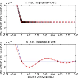
4.1 Non-smooth put payoff function

We first compare the approximation errors of the RBF-interpolation of the (non-smooth) put pay-off (4) using ESM with those using ARSM. To measure the accuracy of our RBF-approximation, we use a set of evaluation points ˆx∆x

i ,

for which we will simply take the grid points ˆ

xi:= ˆx∆xi = ˆxmin+j∆x, jˆ = 1,2, . . . , G. (23)

Here ∆xˆ = (ˆxmax−xˆmax)/G with xmin ≤ xˆmin ≤xˆmax ≤xmax and G is the

number of the evaluation points chosen. We will use the following two norms for the errors, the max error:

E∞(ˆxi, T) =C(1/N)R∞ (24)

for the maximum error and

E2(ˆxi, T) =C(1/N)R2 (25)

for the rms error, where N is the number of interpolation points, C is a con-stant and R2 is the rate of convergence, which is linear when it equals one and

quadratic when it equals two.

In table 1, we compare both types of errors,E∞, in (24) and, E2, in (25) of

ARSM and ESM. As seen in this table, ARSM shows both a lowerE∞ andE2

−0.02−4 −0.01 0 0.01 0.02 0.03 0.04 0.05 0.06 0.07 −2

0 2 4 6x 10

−3

logarithm underlying price, x

Initial condition of Put Function, f(x)

−0.02−4 −0.01 0 0.01 0.02 0.03 0.04 0.05 0.06 0.07 −2

0 2 4 6x 10

−3

Initial condition of Put Function, f(x)

N = 521, Interpolation by EMS N = 521, Interpolation by ARSM

Table 1.E∞ and E2 of the RBF approximation from an initial put function in (4)

using ARSM and those using ESM. G is the number of evaluation points.

ARSM ESM ARSM ESM

G E∞of Put E2of Put

3000 8.8381e-006 0.0022 1.1919e-006 1.1200e-004

4.2 European Option

In this section we present the numerical results of ARSM and ESM, and compare these with both Merton’s analytical option price formula for puts, and with the results of Briani’s finite difference algorithm in Brianiet al.[2]. We use the same formula, (23), to define our evaluation points. We set ˆxmin=K−10 and

ˆ

xmax=K+ 10 whereK is a strike price. Apart from using two error measures,

both (24) and (25), we define two other error measures, the absolute error: Eabs.(x, t) =|V(ex, t)−_bu(x, t)|, (26)

and the relative error:

Erel.(x, t) =

|V(ex_{, t)−}

b

u(x, t)|

V(ex_{, t)} . (27)

whereV(ex_{, t) and}

b

u(x, t) are the exact value and approximate value at the point (x, t).

It is known [25] that the analytical price of a European put option in the Merton Jump-diffusion model is given by

V(S, t) =

∞

X

m=0

e−λ(1+η)τ((λ(1 +η)τ)m

m! VBS(S, τ, K, rm, σm). (28)

whereτ=T−tis the time to maturity,η=eµJ+ σ2_J

2 −1 represents the expected

percentage change in the stock price originating from a jump,σ2

m=σ2+ mσ2_J

τ

the observed volatility,rm=r−λη+mlog(1 +η)/τ andVBSthe Black-Scholes

price of a put, computed as

VBS(S, τ, K, r, σ) =Ke−rτΦ(−d2)−SΦ(−d1) (29)

whereΦ(·) is the cumulative normal distribution and

d1=

log(S

K) + (r+ 1 2σ

2_)τ

σ√τ , d2=d1−σ

p

(τ).

Our RBF-algorithm for numerically solving (3) with initial condition (4) runs as follows:

1. Find the RBF-approximation to the initial value u(x,0) either using ESM or ARSM. This will provide us with a set of interpolation (or collocation) pointsx1, . . . , xn, together with an initial vectorρρρ(0) = ρ1(0), . . . , ρN(0)

2. Then useρρρ(0) as initial value for the system (22). By using any stiff ODE solver, we find out theρρρ(T) at timeT.

3. Finally, substituteρρρ(T) back intoPN

j=1ρj(T)φ(|x−xj|) to get an

approxi-mate value ofu(x, T).

In our numerical experiment we implement the algorithm in MATHLAB R2007b. We select our maximum and minimum logarithm pricexmin log(Smin)

andxmax log(Smax)

, as before, equal to−6 and 6 respectively. By experimen-tation, we do not need as many interpolation points if we restrict the strike price around an interval x∈[−1,1]; therefore, in table 2, we scale down K to K/100. Moreover, we use function quadv which implements recursive adaptive Simp-son quadrature for computing equation (19) as well as function ode23tbwhich implements TR-BDF2 for the calculation of equation (22).

In order to illustrate that ARSM is better than ESM, a comparison ofE∞

and E2 between both methods at increasing time intervals is shown in table 3.

Table 3 shows that the errors in the approximate solution computed using the adaptive ARSM-scheme stay small, even whenT is close to zero, in contrast to the output of the ESM-scheme. Both for ARSM and ESM, the errors increase slowly, if at all, with increasing T, although the errors from using ARSM are much smaller.

In Table 4, we compare the results of the FDM used in Brianiet al.’s paper [2] with those using ARSM and ESM. The ARSM-scheme can achieve lower Eabs(logS) than ARS-233 scheme, Explicit scheme and the ESM-scheme.

Table 5 highlights the accuracy of pricing put values of ARSM and ESM by analysing theirErel.(logS, T) at different timesT and for differentS. Three

par-ticular put prices are examined individually, representing three different cases. Firstly,S= 90 represents the in-the-money case in put. The second,S= 100, is the at-the-money case for a put option, and in the last,S = 110 represents the out-of-the-money case for put options. As before, we choose the first column of the input parameter of table 2 for this experiment.

Figure 2 demonstrates that ARSM gives a smaller Eabs(logS, T), around

6.5×10−4 _{or below, than ESM does. The vertical axis labels ”Abs. Error”}

represents Eabs(logS, T), and the latter is plotted against S and T; S ranges

from 90 to 110 andT from 0 to 1. In our numerical calculations we letSincrease by∆S= 0.1 andT by time-steps of 10e−12_{.From top to bottom, the first graph}

representsEabs(logS) of ARSM and the next one that of ESM. As illustrated in

0 0.2 0.4 0.6 0.8 1 90

95 100 105 1100

2 4 6 8

x 10−4

Time to Maturity, T Stock price, S

Abs. Err.

0 0.2 0.4 0.6 0.8 1

90 95 100 105 1100 0.05 0.1 0.15 0.2 0.25

Time to Maturity,T Stock price, S

Abs. Err.

Table 2.Column 1 input parameters (exceptT = 1e−06,1and 5) are copied from [9] which d’Halluin, Forsyth and Vetzal used to approximate American put options and European call options in 2004. Originally these parameters come from [?] with which Andersen and Andreasen used to calculate European call options on the S&P 500 stock indies in April of 1999. Column 2, input parameters used to value European call and put options under the Merton Jump-diffusion Model. These parameters are copied from [2] which Briani, Natalini and Russo used to price European put and call options in 2007.

Parameter Values

σ 0.15 0.2

r 0.05 0.05

σJ 0.45 0.8

µJ -0.9 0

λ 0.1 0.1

T 1e-06/0.25/1/5 1

K 100 100

Table 3.E∞andE2of a European put option are presented by using input parameters

provided in the first column of Table 2.Gis the number of evaluation points.Tis time-to-maturity.

ARSM ESM ARSM ESM

T G E∞of Put E2 of Put

1e-06 201 7.955929e-05 2.184118e-01 9.862619e-06 8.434566e-02 0.25 201 4.029000e-04 2.277197e-02 2.614984e-04 1.769887e-02 1 201 6.423055e-04 1.047691e-02 4.422346e-04 8.169592e-03 5 201 9.843645e-04 7.308420e-01 6.116825e-04 6.854095e-01

Table 4.Comparative values of a European put option using ARSM and ESM versus those using FDM in Briani’s methods in [2]. Erel.(logS, T) is relative error. S is the stock price. N is the number of interpolation points. Mesh is the number of mesh points. Time-to-maturity, T, is 1.ub(logS, T) is the approximate value of a European put by using ARSM or ESM. Value is approximate value of a European put by using Explicit Scheme or ARS-233 scheme. The parameters are provided in the second column of Table 2.

Explicit scheme ([2]) ARS−233 scheme ([2])

S M esh V alue Erel.(logS, T)M esh V alue Erel.(logS, T) Exact 100 1024 8.319940 2.577970e-03 1024 8.326102 1.839249e-03 8.341436

ARSM ESM

S N u_b(logS, T)Erel.(logS, T) N u_b(logS, T)Erel.(logS, T) Exact 100 521 8.341670 2.804294e-05 1024 8.330652 1.293062e-03 8.341436

4.3 American Put Options

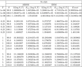
Table 5. Comparison between analytical values of a European put option with its approximate values by using ARSM and ESM.T is the time-to-maturity.ub(logS, T)is the approximate value.Erel.(logS, T)is relative error.Exactis the analytical value of a European put option in (28).N is the number of interpolation points. The parameters are provided in the first column of Table 2.

N=521

ARSM ESM

T S bu(logS, T) Erel.(logS, T) bu(logS, T) Erel.(logS, T) Exact 1e-06 99.9 1.000009e-01 5.885266e-05 5.280614e-02 4.719125e-01 9.999504e-02 1e-06 100.0 5.904871e-03 1.329438e-02 6.849907e-05 9.885538e-01 5.984431e-03 1e-06 100.1 1.138495e-05 1.0543530 -4.661364e-02 8.412183e+03 5.541865e-06

0.25 90.0 9.285133 3.072185e-05 9.272727 1.366755e-03 9.285418 0.25 99.9 3.185076 7.507332e-05 3.185076 6.815555e-03 3.184837 0.25 100.0 3.149258 7.372928e-05 3.127410 6.864284e-03 3.149026 0.25 100.1 3.113936 7.472784e-05 3.092181 6.911995e-03 3.113703 0.25 110.0 1.400927 1.844433e-04 1.394685 4.639699e-03 1.401186

1 90.0 10.303322 6.218437e-05 10.293486 1.016785e-03 10.303963 1 95.0 8.188955 5.814502e-05 8.179676 1.191192e-03 8.189431 1 100.0 6.684307 2.016808e-05 6.676282 1.220705e-03 6.684441 1 105.0 5.653948 7.896656e-05 5.648129 1.108153e-03 5.654395 1 110.0 4.961079 7.478172e-05 4.956963 9.042944e-04 4.961450

5 90.0 15.136039 6.503026e-05 14.566859 3.766688e-02 15.137023 5 95.0 14.200279 5.289616e-05 13.548645 4.593930e-02 14.201030 5 100.0 13.370351 3.583254e-05 12.670378 5.238657e-02 13.370830 5 105.0 12.626235 3.278034e-05 11.902553 5.734664e-02 12.626649 5 110.0 11.952952 2.315001e-05 11.222387 6.114181e-02 11.953229

ARSM and ESM with those of Forysth et al.’s FDM in [9]. As mentioned in section 2, an American put option problem is a free boundary problem because of the possibility of early exercise at any point during its life, leading to the free boundary condition:

u(x, τ) = max K−ex, u(x, τ)

.

Together with the smooth pasting condition mentioned in section 2, this uniquely determines the exercise boundary.

As before, we use both ARSM and ESM to approximateu(x,0) = max(K− ex_{,0) and then continue to work with the interpolation points found atτ = 0.}

The algorithm now reads as follows:

2. Find the RBF-approximation to the initial valueu(x,0) either using ESM or ARSM. This will provide us with a set of collocation or interpolation points x1, . . . , xn, together with an initial vectorρρρ(0) = ρ1(0), . . . , ρN(0)

. 3. Assume we have already determined ρρρ(m∆t) (if m = 0, we have ρρρ(0)) in

equation (22). Solve the system of (stiff) ODEs to findρρρ (m+ 1)∆t

at the next successive time-step, (m+ 1)∆t.

4. Then at time (m+ 1)∆t, for each interpolation pointxi, define

u xi,(m+ 1)∆t= max (K−exi), N

X

j=1

ρj (m+ 1)∆tφ(|xi−xj|).

5. Find a new vectorρρρ (m+ 1)∆tsuch thatu xi,(m+ 1)∆t

=PN

j=1ρj (m+

1)∆t

φ(|xi−xj|) for all i.

6. Repeat Step 3.) to 5.) untilm=M −1. 7. Finally, substituteρρρ(T) back intoPN

j=1ρj(T)φ(|x−xj|) to get an

approxi-mate value ofu(x, T).

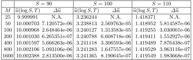
The settings of our numerical experiment are the same as those in section 4.2. In table 6, ∆u_b designates the difference between the values obtained for

b

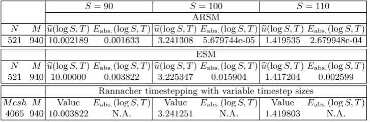
u(logS, T) for two successive values of the number of time-steps, M (listed in the first column of table 6);∆u_bdecreases with increasing number of time-steps. This indicates numerically, at least, that our method converges. In table 7, we use Forsyth et al.’s FDM in [9] as an indicator of the accuracy of our American option prices. Forysth et al.obtain their best results using a scenario involving 4065 mesh points and 940 time-steps. Taking their results as a benchmark for the prices computed using our ESM and ARSM schemes, but with only 521 interpolation points, we see that for the three values of S considered, ARSM gives a much smaller absolute error, Eabs.(logS, T), especially in the

at-the-money and out-of-the-at-the-money cases.

Table 6.Value of an American put option by using ARSM. Number of interpolation points is 521.Mis the number of time-steps._bu(logS, T)is the approximate value of an American option by using ARSM.∆u_bis the change from one level of refinement to the next. Time-to-maturity, T, is 0.25. The parameters are provided in the first column of Table 2.

S= 90 S= 100 S= 110

M _bu(logS, T) ∆u_{b b}u(logS, T) ∆_bu _bu(logS, T) ∆_bu

25 9.999991 N.A. 3.236244 N.A. 1.418371 N.A.

Table 7. Comparison of values of an American put option using ARSM and ESM against those in Forysth et al. [9].N is the number of interpolation points.M is the number of time-steps.M eshis the number of mesh points.V alueis the approximate value of an American option by using Rannacher timestepping with variable timestep sizes.u_b(logS, T) is the approximate value of an American option by using ARSM or ESM.Eabs.(logS, T)is the absolute value of the difference in the pointSof our RBF-solution with that of Forysth et al. [9]. Time-to-maturity, T, is 0.25. The parameters are provided in the first column of Table 2.

S= 90 S= 100 S= 110

ARSM

N M u_b(logS, T)Eabs.(logS, T)u_b(logS, T)Eabs.(logS, T)u_b(logS, T)Eabs.(logS, T) 521 940 10.002189 0.001633 3.241308 5.679744e-05 1.419535 2.679948e-04

ESM

N M u_b(logS, T)Eabs.(logS, T)u_b(logS, T)Eabs.(logS, T)u_b(logS, T)Eabs.(logS, T) 521 940 10.00000 0.003822 3.225347 0.015904 1.417204 0.002599

Rannacher timestepping with variable timestep sizes

M esh M Value Eabs.(logS, T) Value Eabs.(logS, T) Value Eabs.(logS, T)

4065 940 10.003822 N.A. 3.241251 N.A. 1.419803 N.A.

5

Conclusions

We have implemented a RBF method to solve the PIDE boundary value problem for pricing American and European put options on a non-dividend-paying stock in a Merton jump-diffusion market [25]. We also compared ARSM and ESM for determining RBF-interpolation points. Our results suggest that one can achieve a high accuracy by implementing ARSM which involves a limited number of interpolation points. Moreover, several drawbacks associated with grid-based methods like the FDM have been avoided: we do not have to make assumptions on the behavior of the solutions outside of the solution domain, we seem to avoid the stability problems associated with explicit or implicit finite difference schemes. Moreover, we dramatically improve the accuracy of pricing put options in particular for small times to maturity, by implementing ARSM.

References

1. Andersen, L. and Andreasen, J., 2000. Jump-diffusion Processes: Volalitility Smile fitting and Numerical Methods for Option Pricing.Review of Derivatives Research, 4, pp. 231 - 262.

2. Briani, M., Natalini R. and Russo, G., 2007. Implicit-explict Numerical Schemes for Jump-diffusion Processes.Calcolo, 44, pp. 33–57.

4. Buhmann. M. D., 2003.Radial basis functions: theory and implementations, vol-ume 12 of Cambridge Monographs on Applied and Computational Mathematics. Cambridge University Press, Cambridge.

5. Brummelhuis, R. and Chan R. L. T., 2014. A radial basis function scheme for option pricing in exponential Lvy models.Applied Mathematics Finance, 21:3, pp. 238–269.

6. Chan, R. L.T. and Hubbert, S., 2014. Options pricing under the one-dimensional Jump-diffusion model using the radial basis function interpolation scheme.Review of Derivatives Research,17:2, pp. 161–189.

7. Cont, R. and Voltchkova, E., 2005. A Finite Difference Scheme for Option Pricing in Jump Diffusion and Exponential L`evy Models. SIAM Journal on Numerical Analysis, 43, pp. 1596 - 1626.

8. Cont, R. and Tankov, P., 2004.Financial Modelling With Jump Processes, CHAP-MAN & HALL/CRC Finanical Mathematics Series.

9. d’Halluin, Y., Forsyth, P.A. and Vetzalz, K.R., 2005. Robust Numerical Methods for Contingent Claims under Jump Duffusion Process.IMA J. Num. Anal., 25, pp. 87 - 112.

10. d’Halluin, Y., Forsyth, P.A. and Labahn, G., 2004. A Penalty Method for American Options with Jump Diffusion Processes.Numerische Mathematik, 97(2), pp. 321 -352.

11. Driscoll, T. A. and Heryudono, A., 2007. Adaptive Residual Subsampling Meth-ods for Radial Basis Function Interpolation and Collocation Problems.Computers Math. Appl., 53, pp. 927 - 939.

12. Fasshauer, G. E., Khaliq, A. Q. M. and Voss, D. A., July, 2004. A Parallel Time Stepping Approach Using Meshfree Approximations for Pricing Options with Non-smooth Payoffs. Proceedings of Third World Congress of the Bachelier Finance Society, Chicago.

13. Fasshauer, G. E. and Zhang, J. G.. On Choosing Optimal Shape Parameters for RBF Approximation.To be appeared in Numerical Algorithms.

14. Fasshauer, G. E., Khaliq, A. Q. M. and Voss, D. A., 2004. Using Meshfree Approxi-mation for Multi-Asset American Option Problems.J. Chinese Institute Engineers, 27(4), pp. 563 - 571.

15. Fornberg, B. and Wright, G., 2004. Stable Computation of Multiquadric Inter-polants for All Values of the Shape Parameter.Comput. Math. Appl., 47, pp. 497 - 523.

16. Hon, Y.C. and Mao, X. Z., A Radial Basis Function Method for Solving Options Pricing Model.Financial Engineering, to appear.

17. Hull, J.C., 2007.Options, Futures, and Other Derivatives, Seventh Edition, Pearson Education.

18. Johnson, C., 1987. Numerical Solutions of Partial Differential Equations by the Finite Element Method.Cambridge University Press, Cambridge.

19. Kansa, E. J. and Carlson, R. E., 1992. Improved Accuracy of Multiquadric Inter-polation Using Variable Shape Parameters. Comput. Math. Applic., 24, pp. 99 -120.

20. Kansa, E. J. and Carlson, R. E., 1994. The Laplace Transofrm Multiquadrics Method: A Highly Accurate Scheme For The Numerical Solution of Linear Partial Differential Equations.Journal of Applied Science & Computations, 1(2), pp. 375 - 407.

22. Kansa, E. J., 1990. Multiquadrics-A Scattered Data Approximation Scheme with Applications to Computational Fluid-Dynamics-II: Solutions to Parabolic, Hyper-bolic and Elliptic Partial Differential Equations. Comput. Math. Appl., 19(8/9), pp. 147 - 161.

23. Madan, D.B. and Seneta, E., 1990. The Variance Gamma (V.G.) Model for Share Market Returns.Journal of Business, 63, pp. 511 - 524.

24. Matache, A., Schwab, C. Wihler, T. P., 2005. Fast Numerical Solution of Parabolic Integrodifferential Equations with Applications in Finance.SIAM Journal on Sci-entific Computing, 27(2), pp. 369 - 393.

25. Merton, R. C., 1976. Option Pricing when Underlying Stock Returns are Discon-tinuous.Journal of Financial Economics, 3, pp. 125 - 144.

26. Pham, H., 1997. Optimal Stopping, Free Boundary, and American Option in a Jump-diffusion Model.Appl. Math. Optim., 35, pp. 125 - 144.

27. Powell, M. J. D., 1992. The Theory of Radial Basis Function Approximation in 1990, in: W. Light (Ed.).Advances in Numerical Analysis, II: Wavelets, Subdivision Algorithms and Radial Basis Functions, Clarendon Press, Oxford, pp. 105 - 210. 28. Rannacher, R., 1984. Finite Element Solution of Diffusion Problems with Irregular

Data.Numerische Mathematik, 43, pp. 309 - 327.

29. Sarra, S. A., 2005. Adaptive Radial Basis Function Methods for Time Dependent Partial Differential Equations.Applied Numerical Mathematics, 54(1), pp. 79 - 94. 30. Schoutens, W., 2006. Exotic Options under L´evy Models: an Overview.Journal of

Computational and Applied Mathematics, 189, pp. 526 - 538.

31. Shampine, L. F., 2008. Vectorized Adaptive Quadrature in MATLAB.Journal of Computational and Applied Mathematics, 211(2), pp. 131 - 140.