3307
SWITCHING BOND GRAPH APPROACH FOR STRUCTURAL
CONTROLLABILITY OF SWITCHED LINEAR SINGULAR
SYSTEMS
1MOHAMED BENDAOUD, 2HICHAM HIHI, 3KHALID FAITAH
1LGECOS Laboratory, National School of Applied Sciences, Marrakech, Morocco
2Department of Electrical Engineering, Cadi Ayad University, Marrakech, Morocco
3Department of Electrical Engineering, Cadi Ayad University, Marrakech, Morocco
E-mail: 1 [email protected], 2[email protected], 3[email protected]
ABSTRACT
This paper investigates the structural controllability of switched linear singular systems (SLSS). Graphical methods are proposed in order to determine different conditions for the structural controllability of SLSS systems. These methods are based on simple causal paths and causal manipulations on the switching bond graph model. Our approach can be implemented in software such as Symbol2000 or 20sim, in order to control the systems in real time.
Keywords: Singular System, Switched Systems, Bond Graph, Structural R-Controllability, Structural I-Controllability, Structural C-Controllability.
1. INTRODUCTION:
Switched systems are frequently encountered in practice, for example (hydraulic systems with valves, electric systems with diodes, relays, mechanical systems with clutches...). It is for this reason that various researchers have approached the study of controllability/observability for this systems, and a lot of results have emerged during the twenty last years with different approaches (algebraic, graphical...) [1]–[6].
Some sufficient conditions and necessary conditions for controllability of hybrid system were presented in [3], where the system operating period within each mode was assumed to be fixed and known. Complete geometric criteria for controllability and reachability are established in [1], [2]. Some necessary and sufficient conditions for controllability are derived in [4], [5]. The observability of the continuous and discrete states of hybrid systems are studied in [6], [7].
The switched linear singular systems are an important class of switched systems. Due to the existence of switching, discontinuity phenomenon appears in the state variables at the switching moments. Physically, some problems such as sparks and short circuits can occur. Therefore the stability, controllability and observability of switched
singular systems are important research topics in the area of switching control. Little works have been done on the controllability of switched linear singular systems. In [8] and [9], the solvability and controllability of periodically switched singular systems were studied. By using the geometric approach, a necessary condition and a sufficient condition on complete reachability are presented in [10].
Up to now, all previous work mentioned above has been based on the traditional controllability concept, for example in [10] the conditions proposed require a lot of matrix calculates to check controllability, Hence it is desirable to investigate controllability and observability by structural properties and not by the parameter numerical values, this properties are independent of the numerical value of the system and depending only on the architecture of the system.
3308 these systems [15]–[22], based on simple causal manipulations on the bond graph model.
The controllability and observability study of linear time invariant system (LTI) is based on two fundamental notions: attainability and structural rank, the latter is determined directly from the bond graph model [20], [21].
When switched linear system has just one mode, it can be considered as a LTI system. So we can therefore apply the same results obtained for the LTI systems. In this context some necessary and sufficient conditions for controllability and observability for switched systems are derived in [18], [19], with the aid of simple causal manipulations on the switching bond graph (SBG).
On the other hand, the controllability property is decomposed into R-controllability, impulse controllability and complete controllability [23]. For R-controllability of switched singular systems, we proposed some conditions using simple causal manipulations on the bond graph model in [24].
In this paper, we investigate the structural controllability problem for switched linear singular systems modeled by switching bond graph. Unlike the other approaches (algebraic) [8]–[10], the results obtained in this work are more applicable since the conditions developed in this paper are based on simple causal manipulations on the bond graph model, which not only avoids lot of matrix calculates but can also check controllability without knowing the system parameters.
This paper is organized as follows: the second section formulates algebraic results related to the analysis of controllability. Section three recalls some background about bond graph modelling of switched systems. The modelling is done using the structure junction equation, leading to an implicit model. In section four, graphical methods for structural R-controllability, I-controllability and C-controllability of these systems are proposed. This procedure is based on simple causal manipulations on the bond graph model. Finally, a simple example illustrating the previous results is proposed.
2. ALGEBRAIC ANALYSIS OF THE CONTROLLABILITY
2.1. System description and preliminaries
Considering a switched linear singular system, given by equation (1):
(1)
Where ∈ , ∈ , and ∈ are
respectively the state, input and output vectors.
If we consider this system in a particular mode , the equation (1) can be written as:
(2)
With , ,
, , ∈ 1, … , and is the
number of modes.
2.2. Decomposition of the singular system
It is usual, when analyzing the properties of (2), define equivalent forms by pre-multiplying it by a non-singular matrix P, and by operating a variable
change in order to obtain a new equivalent implicit state equation [23]:
Such that 0 0
0 0 and
Introducing the state transformation:
̅
Using (4), the equivalent canonical form of equation (2) can be defined as:
a b
c
The equation (5) usually called Kronecker form. The subsystems (5.a) and (5.b) are called slow and fast subsystems respectively.
∈ and ∈ are the slow and
3309 The Kronecker form separates the finite dynamic modes from pulse and non-dynamic modes, and solves each of the subsystems separately.
2.3. R-controllability of SLSS system in a particular mode
When system (1) has just one mode, it can be considered as a singular LTI system, and we consider the equivalent form of Kronecker-Weierstrass [23].
Thus, the slow subsystem (5.a) is an ordinary differential equation. It has a unique solution for any piecewise continuous input and an initial condition 0 , given by (6).
0 (6)
The slow subsystem is controllable if and the controllability matrix defined as
… .
Definition 1 [23]: R-controllability is related to the ability to control the finite dynamic modes (classical controllability of exponential modes for regular system). It is associated with the differential part composing the state space.
The R-controllability guarantees our controllability for the system from any admissible initial condition 0 to any reachable state and this process will be finished in any given time period if the control is suitably chosen.
Theorem 1[23]: The system (2) in a particular mode j is called R-controllable, if the slow subsystem (5.a) is controllable.
2.4. R-controllability of SLSS system with q modes
We can define a combined matrix of SLSS system as:
… … (7) With is the controllability matrix in mode . Theorem 2(Extension of Yang’s Theorem): The SLSS with modes is R-controllable; if the controllability matrix defined in (7) is of full
row rank, i.e. .
Proof of theorem 2: See the Appendix.
□
Remark 1: From theorem 2, we can deduce that: - The system (1) can be R-controllable, if the system (2) in a particular mode is R-controllable.- However, it is possible that no mode is R-controllable but the system (1) is R-R-controllable.
2.5. Impulse controllability
There exist impulse terms that is set out either by the initial condition or by the possible jump behavior in control input and its derivatives. Therefore, it is necessary to analyze the control effect on impulse terms in the stale response. Definition 2: Impulse controllability is important for the necessity to eliminate the impulse portions in a system in which impulse terms are generally not expected to appear.
Theorem 3 [23] : The system (2) in a particular mode j is called I-controllable, if the fast subsystem (5.b) is controllable.
2.6. C-controllability
Definition 3 [23]: The system (2) in a particular mode is called C-controllable, if both its slow and fast subsystems are controllable.
3. REPRESENTATION OF A LINEAR
SINGULAR SYSTEM FROM A
SWITCHING BOND GRAPH
[image:3.612.315.517.455.618.2]The structure junction of a switching bond graph (SBG) can be represented by figure 1.
Figure 1: Junction structure of a switching bond graph
Five fields model the components behavior: - source field which produces energy, - R field which dissipates it, - I and C field which can store it, -
and continuous detectors fields, and the Sw field
is the switching component. These elements are linked directly to the control system discrete.
The continuous part of system
The discrete part of system
Source field
R
Integral
causality Structure Junction (0,1,MTF,M
GY)
Switch field (Sw)
Spontaneous transitions
Continuous detectors
,
Derivative causality
3310 is the state vector. It contains the variables p on I
elements and the variables q on C elements when
these elements are in integral causality. is the pseudo state vector: it contains the variables p on I
elements and the variables q on C elements when
these elements are in derivative causality. and are vectors that contain the coenergy variables associated to and . and contain the effort and flow variables respectively entering and exiting from resistive ports. and are vectors that contain the variables respectively imposed and exiting from switches in mode .
3.1. Bond graph models of switch and switched sources elements
The switch elements can be modelled using two main bond graph approaches: non ideal switches [16] or ideal switches [15]. In the second case, the sources standing for ideal switches have two states (figure 2): the first state denoted by ON, when they behave like zero effort sources ( : 0) and a second state denoted by OFF when they behave like zero flow sources ( : 0). These two sources represent the discrete inputs and are noted , they can be efforts or flows entering in structure of junction. For a system contain N switchs, we need to define the discrete sources by:
, ∈ 1, ⋯ , , ∈ 1, ⋯ , with
[image:4.612.315.519.192.344.2]2 those define the set of discrete inputs, and are presented in Figure 2.
Figure 2: Bond graph models of switched sources and
3.2. State representation from switching bond graph
Each output of the junction structure ,
, , and can be expressed
as function of all its inputs ,
, , , and :
0 0
0
This linear relation can be written as an implicit equation that is called in the following the standard implicit form:
0 0
0 0
0 0
Where
0
0
0 0 0
0 0 0
0 0 0
0
0 0
0 0 0
Matrices , S , and are skew symmetric due to energy considerations.
Let the constitutive law of the field be: .
is a positive matrix, with 0
0 1/
0 or 1
Sw
a) Spontaneous commutation Internal discrete event
: :
0 or 1
Sw
b) Controlled commutation External
discrete event
3311
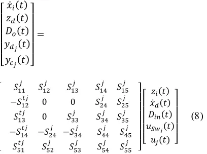
If S exists, which is particularly
true when is a symmetric and positive definite matrix, then third row of (8) leads to:
S S S
By eliminating and from (8) we obtain the equation (11):
0 0
0
0
0
Where
and
In a linear case, the law constitutive for the fields of storage and can be written as:
0
0
Where 1/0 1/0 and 0
0
In mode , we have 0, so for ∈ , the state representation is given by:
Where
,
0 0 0 0 ,
0 0
, ,
, 0 0
, ,
, 0 0
Where ∈ and ∈
Thus, for a system with switches, the number of modes is given by 2 . The hybrid system evolves by according to the following dynamical:
∈ ,
⋮
∈ , 13
⋮
∈ ,
3.3. Decomposition of the singular system
To go further in the analysis of the implicit equation (12), it is pre-multiplied by the nonsingular matrix:
0
0
0
Where
Defining also the variable change:
Where
0
0
Leads to the following explicit state representation: 0
0 0 0 0
Equation (17) is equivalent to an ordinary state representation:
(18) Where the state is continuous at the origin, associated to an algebraic equation:
(19)
Where =
3312 3.4. Determination of the equivalent bond
graph of slow subsystem
The following procedure shows the symbolic calculation of the equivalent ordinary state representation (18) for linear singular systems directly from their bond graph model.
components of vector are calculated so as to reduce the components of the vector (which are causally connected to an element of the vector ) to the components of the vector t extracted by equation (15) :
(20)
Changing the t elements by t element in bond graph model. To explain that, we propose the following example:
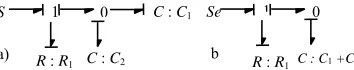
Example 1: We consider the bond graph model given by Figure 3.a and its equivalent bond graph (EBG) model given by Figure 3.b.
Figure 3 a) BGI, b) Equivalent bond graph model (EBGI)
Where
t (21)
Note that
(22)
Then, we obtain the relations:
and (23) So the EBG of slow subsystem is found by changing the value of through and by removing the element in derivative causality. Physically, we can explain that by the existence of an equivalent C-element, which groups the two elements in parallel.
and are obtained by causal manipulations on the EBGIj model of slow subsystems and, they are given by the following propositions:
Proposition 1[24]: In the -matrix, the
-term is obtained by expression (24).
( ∑ ∈ , (24) Where ∈ 1, … , , ∈ 1, … , , ∈ 1, … , .
, is the causal path gain of length
1from to .
is the gain of the I or C element in integral causality associated with : and
.
Proposition 2[24]: In the -matrix, the term
is obtained by expression (25):
∑ ∈ , (25)
Where ∈ 1, … , , ∈ 1, … , and ∈
1, … , .
, is the constant term of the gain of the causal path of generalized length from the (Se
or Sf ) associated with to dynamical element (I,C) in integral causality associated with .
4. STRUCTURAL CONTROLLABILITY
The objective of this part is to present graphical methods using the bond graph methodology to derive information on structural controllability. For the SLSS, the controllability property is decomposed into R-controllability, impulse controllability and complete controllability. In the following, EBGI and EBGD denote respectively the equivalent bond graph model of slow subsystem when the preferential integral (respectively derivative) causality is affected.
4.1. R-controllability
- Graphical sufficient condition 1
To study structural R-controllability of switched singular system modeled by switching bond graph, we must for each mode, transform it to an equivalent bond graph of the slow subsystem. Therefore, we can therefore apply the same results obtained for the LTI systems.
Proposition 3: In a particular mode , the slow
subsystem (18) is structurally controllable if: 1- All dynamic elements in integral causality are causally connected with a continuous input control.
2- , with ∈ 1, … , }.
Proof of proposition 3: This result is derived from
digraph theory [25].
□
Property 1: .
1 0 C : C1
S
a) R : R
1
1 0
Se
b
R : R1 C : C1 +C2
[image:6.612.105.282.354.389.2]3313 Where is the number of elements remaining in integral causality in EBGDj, when a dualism of the maximum number of continuous input sources is applied (in order to eliminate elements in integral causalities). And is the number of element in integral causality in EBGIj.
Proof of Property 1 : After transformation of
switched singular system modeled by switching bond graph, to an equivalent bond graph of the slow subsystem, the proof of this property is equivalent to the one proposed in the case of switched systems [21].
□
On the other hand, the switched linear singular system (12) in a particular mode is called R-controllable, if the slow subsystem (18) is controllable. Hence to study the R-controllability of system (1), it is necessary to apply this result to all modes; if one controllable mode exists, the procedure is stopped. The case where no mode is R-controllable, but the system (1) is R-R-controllable, Therefore the sufficient condition 1 cannot be applied in this case, where the interest of the proposed condition below.
- Graphical sufficient condition 2
After transformation of switched singular system modeled by switching bond graph, to an equivalent bond graph of the slow subsystem, we can apply the proposed procedure in [22], in order to calculate the subspace of structural controllability of each mode , noted .
On the EBGDj when a dualization of the maximum number of continuous input sources is applied (in order to eliminate elements in integral causalities), we can write for each element I and C remaining in
integral causality algebraic equations:
∑ 0 (26)
is either an effort variable for I-element in
integral causality or a flow variable for C
-element in integral causality.
is either an effort variable for I-element in
derivative causality or a flow variable for C
-element in derivative causality.
is the gain of the causal path between the I
or C-elements in integral causality and the I or C-elements in derivative causality.
Let us consider the row vectors 1, … , whose components are the coefficients of the variables , in the equation (26).
Property 2: The row vectors 1, … , are
orthogonal to the structural controllability subspace vectors of the mode. We write ,…,
and . With is uncontrollable
subspace in mode , used to check orthogonality. In the same way, from the EBGDj (with dualization of inputs sources), we can write for each element I
and C remaining in derivative causality
algebraic equations:
∑ 0 (27)
is either a flow variable for I-element in
derivative causality or an effort variable for C-
element in derivative causality.
is either a flow variable for I-element in
integral causality or an effort variable for C
-element in integral causality.
is the gain of the causal path between the element in derivative causality and the element in integral causality.
Now, we consider the column vectors whose components are the coefficients of and variables in equation (27).
Property 3: n t column vectors w r 1, … , n t compose a basis for the structural R-controllability subspace of j mode. With
,…, and .
Proof of Property 3: Equations (26) and (27) provide dual algebraic relations. So we can easily verify that 0.
□
Now, we can define a combined matrix of
SLSS system as: … … .
With ,…, is the controllability
matrix of mode.
Using the graphical calculation of structural controllability subspaces and theorem 2, the following theorem is proposed.
Theorem 4: If , the switched
linear singular system (1) is structurally R-controllable.
3314 We have shown for a given mode that the EBGDj (with dualization of inputs sources) is characterized by an algebraic equation (27). From this equation we build a basis for the structural R-controllability subspace of j mode. With
,…, and . In the same way,
we build … … , with
,…, for all mode.
However, the condition of Theorem 2 is sufficient for the controllability of the system, which implies
that the condition is also
sufficient.
□
4.2. Impulse controllability
Proposition 4 [19]: A SLSS system is impulse controllable if and only if the number of impulse modes is equal to the number of disjoint causal paths between input sources and switches passing through (I,C) elements in derivative causality in the
BGIj.
_ _ (28)
- represents causal paths between (I,C)
elements in derivative causality and switches elements and _ is equal to the number of impulse modes.
- is the input sub-matrix connecting input sources and (I,C) elements in derivative
causality in the BGIj,
- is composed by causal paths between input sources and switches passing through elements in derivative causality in the BGIj.
So _ corresponds to the
number of disjoint causal paths between input sources and switches passing through elements in derivative causality.
5. EXAMPLE
[image:8.612.317.521.225.425.2]We consider the following acausal switching bond graph model (Figure 4):
Figure 4: Acausal switching bond graph model
This switching bond graph model contains two switches (Sw1 and Sw2), so four modes are
possible, but only three are considered: Mode 1 (Sw1 open, Sw2 closed), Mode 2 (Sw1 closed, Sw2
closed), Mode 3 (Sw1 closed, Sw2 open).
There are five state variables ( , , , , ), one element in derivative causality ( ) and four element in integral causality ( , , ). The
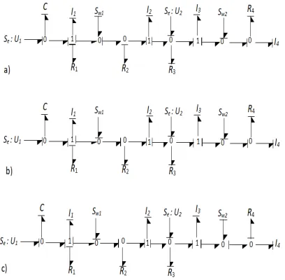
switching bond graph models in integral causality for these three modes are given in figure 5.
Figure 5: Switching bond graph model in integral causality for a) mode 1, b) mode 2, c) mode3
3315 Figure 6 : EBGIj for a) mode 1, b) mode 2, c) mode 3
The application of the derivative causality and dualisation of these modes are given in Figure 7:
[image:9.612.96.319.211.380.2]
Figure 7 : EBGDj+dualisation a) mode 1, b) mode 2, c)
mode 3
Application of graphical sufficient condition 1 i. On the EBGI , all the elements in integral
causality are connected with a continuous input control, and on the EBGD , one element stays in integral causality (Figure 6.a), and the dualization of inputs sourcesdoes not change its causality. So this mode is not R-controllable.
ii. On the EBGI , all the elements in integral causality are connected with a continuous input control, and on the EBGD , two elements stays in integral causality and (Figure 6.b), and the dualization of inputs sourcesdoes not change its causality. So this mode is not R-controllable.
iii. On the EBGI , all the elements in integral causality are connected with a continuous input control, and on the EBGD , one element stays in integral causality (Figure 6.c), and the dualization of inputs sourcesdoes not change its causality. So this mode is not R-controllable.
Since no mode is controllable, we apply the second graphical sufficient condition:
Application of graphical sufficient condition 2 i. In the EBGD (Figure 7.a), remain in
integral causality, we can write 0, thus 0 0 0 1 . The dynamic elements , ,
and are not causally connected with . So f f f 0. The three corresponding
vectors are 1 0 0 0 ,
0 1 0 0 and 0 0 1 0 .
We have 0, then
and ,
with 3
ii. In the EBGD (Figure 7.b), and remain in integral causality, we can write 0,
thus 0 0 0 1 . And 0 thus
0 1 1 0 . The algebraic equations corresponding to and are given by:
0 and 0. then 1 0 0 0
and 0 1 1 0 .
We have 0, then
and , with 2 .
iii. In the EBGD (Figure 7.c), The element is in integral causality and causally connected with and , we can write
0, thus 0 1 1 1 . The algebraic equations corresponding to , and are
given by : 0, 0 and
0. The three corresponding vectors are
w 1 0 0 0 , w 0 1 0 1 and
0 0 1 1 .
We have 0, then
and ,
with 3
From theorem 4 we have:
1 0 0 ⋮ 1 0 ⋮ 1 0 0
0 1 0 ⋮ 0 1 ⋮ 0 1 0
0 0 1 ⋮ 0 1 ⋮ 0 0 1
0 0 0 ⋮ 0 0 ⋮ 0 1 1
4
Then the system is R-controllable. Impulse controllability
Four all mode, element in derivative causality ( ) is not causally connected with the switches Sw1 and Sw2 so, the number of impulse modes equal to 0.Then according to proposition 4 the system is
3316 The system is structurally R- controllable and Impulse controllable then the system is structurally C- controllable.
6. CONCLUSION
In this paper, we have shown a very simple graphical method, based on the manipulation of the causal path leading to the determination of the equivalent explicit state equation of the singular state equation. From this result we have been able to extend the procedures of controllability analysis of switching systems to SLSS. On the other hand the controllability property is decomposed into R-controllability, impulse controllability and complete controllability. For that we have proposed two sufficient graphical conditions for R-controllability, and a procedure that allows an easy determination of impulse modes from a bond graph model. This procedure is based on simple causal manipulations on the equivalent bond graph model in integral and derivative causality. Finally, we have proposed a simple example illustrating our results.
The bond graph model appears to be an excellent tool for structural analysis, through its graphic character and its causal structure. It provides directly to the user information about controllability and observability, sometimes difficult to obtain by other routes.
The second graphical sufficient condition that we have proposed in this paper is limited to the case when all storage elements keep their initial causality during the commutation. Therefore, in our next work, we will take into consideration the changes of causality in the storage elements at the commutation time.
Other aspects which remain to be investigated are: -proposition of a feedback control of finite mode (slow subsystem) -compensation of infinite modes (fast subsystem), in the case where the system is impulse controllable.
Appendix A. Proof of Theorem 2
The proof is similar to that of Yang’s theorem in [4] We consider the slow subsystem (5.a) and we assume that the is invariable for all mode, i.e. with ∈ 1, … , 1 . Going through all the modes with
⋯ the continuous state at can be expressed as:
…
…
⋯ (A.1)
Note that . Then, from (A.1) we can obtain the relation:
̅
… (A.2)
For 1, … , 1 we define :
… (A.3)
Such that , where denotes the unitary matrix.
So the equation (A.1) can be transferred into:
̅
… (A.4)
For term of (A.4) we define:
(A.5)
On the other hand, the exponential matrix can be expressed as [26]:
⋯ ∑ (A.6)
Divide interval , into subintervals, with
property , , ⋯ , . It is noted
that , and , . And we can
define the piecewise continuous input as a piecewise constant function, denoted as
, for ∈ , , , where , ∈ for 1,2, … . , . Substitute the above-defined input and equation (A.6) into (A.5), then we have:
(A.7)
Where … ,
,
, ⋯
, ,
⋮ ⋱ ⋮
,
, ⋯
, ,
,
and
,
⋮
3317
Where for 0,1, … , 1 are the
expansion coefficients of as shown in (A.6). By following the same process, equation (A.4) can be expressed as:
̅ ⋯
⋯
⋯ 0
⋮ ⋱ ⋮
0 ⋯ ⋮ (A.8)
Denote for 1, … , then with
respect to (A.3), we have lim
,.., → .
When for 1, … , are small enough, we can get:
⋯ ⋯ (A.9)
Considering the assumption that the controllability matrix is of full row rank, then we have
⋯ .
Summing up the above analysis, we can see that there exists a timed mode-switching sequence , , , , and a corresponding piecewise continuous input signal , for ∈
, , , with 1, … , and 1, … , , they make hybrid state ; reachable from ; within period ; . Here, the proper selection of , for 1, … , 1 makes the corresponding nonsingular; the proper selection
of , for 1, … , makes condition (A.9)
satisfied and the assignment of , is the corresponding solution of (A.8) when
and .
REFERENCES
[1] Z. Sun, S. S. Ge, and T. H. Lee, “Controllability and reachability criteria for switched linear systems,” Automatica, vol.
38, pp. 775–786, 2002.
[2] G. Xie and L. Wang, “Controllability and stabilizability of switched linear-systems,”
Syst. Control Lett., vol. 48, no. 2, pp. 135–
155, Feb. 2003.
[3] J. Ezzine and A. H. Haddad, “Controllability and observability of hybrid systems,” Int. J. Control, vol. 49, no. 6, pp.
2045–2055, Jun. 1989.
[4] Z. Yang, “An algebraic approach towards the controllability of controlled switching linear hybrid systems,” Automatica, vol. 38,
no. 7, pp. 1221–1228, 2002.
[5] G. Stikkel, J. Bokor, and Z. Szabó, “Necessary and sufficient condition for the controllability of switching linear hybrid systems,” Automatica, vol. 40, no. 6, pp.
1093–1097, 2004.
[6] R. Vidal, A. Chiuso, S. Soatto, and S. Sastry, “Observability of linear hybrid systems,” Hybrid Syst. Comput. Control. Proc., vol. 2623, pp. 526–539, 2003.
[7] E. De Santis, M. D. Di Benedetto, and G. Pola, “On observability and detectability of continuous-time linear switching systems,” in 42nd IEEE International Conference on Decision and Control (IEEE Cat. No.03CH37475), 2003, vol. 6, pp. 5777–
5782 Vol.6.
[8] J. Sreedhar and P. Van Dooren, “Periodic descriptor systems: solvability and conditionability,” IEEE Trans. Automat. Contr., vol. 44, no. 2, pp. 310–313, 1999.
[9] B. Cantó, C. Coll, and E. Sánchez, “Positive N-periodic descriptor control systems,” Syst. Control Lett., vol. 53, no. 5,
pp. 407–414, 2004.
[10] B. Meng and J.-F. Zhang, “Reachability conditions for switched linear singular systems,” IEEE Trans. Automat. Contr.,
vol. 51, no. 3, pp. 482–488, 2006.
[11] C.-T. Lin, “Structural controllability,” IEEE Trans. Automat. Contr., vol. 19, no. 3, pp.
201–208, 1974.
[12] R. Shields and J. Pearson, “Structural controllability of multiinput linear systems,” IEEE Trans. Automat. Contr.,
vol. 21, no. 2, pp. 203–212, 1976.
[13] K. Glover and L. Silverman, “Characterization of structural controllability,” IEEE Trans. Automat. Contr., vol. 21, no. 4, pp. 534–537, 1976.
[14] X. Liu, H. Lin, and B. M. Chen, “Structural controllability of switched linear systems,”
Automatica, vol. 49, no. 12, pp. 3531–3537,
2013.
[15] J. Buisson, “Analysis of switching devices with bond graphs,” J. Franklin Inst., vol.
330, no. 6, pp. 1165–1175, 1993.
[16] G. Dauphin-Tanguy and C. Rombaut, “Why a unique causality in the elementary commutation cell bond graph model of a power electronics converter,” in
Proceedings of IEEE Systems Man and Cybernetics Conference - SMC, 1993, pp.
257–263 vol.1.
3318 “Modelling and structural observability of switching linear hybrid singular systems,”
Int. J. Model. Identif. Control, vol. 27, no.
4, pp. 279–292, 2017.
[18] H. Hihi, “Structural controllability of switching linear systems,” J. Comput., vol.
4, no. 12, pp. 1286–1293, 2009.
[19] A. Rahmani and G. Dauphin-Tanguy, “Structural analysis of switching systems modelled by bond graph,” Math. Comput. Model. Dyn. Syst., vol. 12, no. 2–3, pp.
235–247, 2006.
[20] C. Sueur and G. Dauphin-Tanguy, “Structural controllability/observability of linear systems represented by bond graphs,”
J. Franklin Inst., vol. 326, no. 6, pp. 869–
883, 1989.
[21] C. Sueur and G. Dauphin-Tanguy, “Bond-graph approach for structural analysis of MIMO linear systems,” J. Franklin Inst.,
vol. 328, no. 1, pp. 55–70, 1991.
[22] C. Sueur and G. D. Tanguy, “Bond graph determination of controllability subspaces for pole assignment,” in Proceedings of IEEE Systems Man and Cybernetics Conference - SMC, 1993, pp. 14–19 vol.1.
[23] L. Dai, Singular Control Systems, no. 118.
Springer-Verlag Berlin Heidelberg, 1989. [24] M. Bendaoud, H. Hihi, and K. Faitah,
“Graphical conditions for R-controllability of generalized linear switching systems,” in
2014 International Conference on Control, Decision and Information Technologies (CoDIT), 2014, pp. 459–464.
[25] K. J. Reinschke and G. Wiedemann, “Digraph characterization of structural controllability for linear descriptor systems,” Linear Algebra Appl., vol. 266,
no. Supplement C, pp. 199–217, 1997. [26] W. J. Rugh, Linear system theory (2nd ed.).