Enhancement fuzzy goal programming approach for multi item/ multi supplier selection problem ina fuzzy environment

ORIGINAL RESEARCH ARTICLE

ENHANCEMENT FUZZY GOAL PROGRAMMING APPROACH FOR MULTI- ITEM/ MULTI- SUPPLIER

SELECTION PROBLEM INA FUZZY ENVIRONMENT

*1

_{Khalifa, H. A. and}

2

_{Al- Shabi, M.}

1

_{Department of Operations Research, Institute of Statistical Studies and Research, Cairo University, Giza, Egypt}

2

_{Department of Management Information System, College of Business Administration,}

Taibah University, Saudi Arabia

ARTICLE INFO ABSTRACT

Supplier selection problem (SSP) is one of the important elements in supply chain management which provides a better decision tool for the selection of the supplier. In this paper, a multiple sourcing supplier selection (F-SSP) problem is introduced as a fully fuzzy multi- objective linear programming problem. While the F-SSP is converted into the corresponding



-SSP based on the





cut of the fuzzy numbers, an interactive fuzzy goal programming approach is applied to obtain the



- best compromise solution. The solution procedure controls the search direction via updating both the membership values and the aspiration levels, where the decision maker's role is concentrated only in evaluating the



- efficient solution. Finally, a numerical example is given to the utility of our solution procedure.

Copyright © 2018, Khalifa and Al- Shabi. This is an open access article distributed under the Creative Commons Attribution License, which permits unrestricted use, distribution, and reproduction in any medium, provided the original work is properly cited.

INTRODUCTION

Supplier selection is complicated real world problem due to the ambiguity, uncertainty, imprecise, and vagueness of the data, and is considered as the main concern of modern companies in highly competitive environments. Supplier selection needs to analyze a number of suppliers on many objectives which are often extremely conflicting (Davari et al. 2008). Supplier selection have become important due to the increasing strategies role that supplies play in a buying firm's competitive landscape (Narasimhan and Talluri, 2009). Xia and Wu, 2007 introduced two types of supplier selection problems as single and multiple sourcing. Amid et al. 2006, and Weber and Current, 1993 introduced a multi- objective mixed integer programming model for supplier selection and order allocation among the selected suppliers. Mendoza et al., 2008 designed a new multi-criteria method to solve the general supplier selection problem. He et al. 2009 studied a VSP in which the buyer allocates achieved at minimum cost. Ware et al. 2012 provided an extensive state-of-the-art literature review and critique of the studies related to various aspects of supplier selection problem over the past two decades. Ekhtiari and Poursafary, 2013 studied the process of selecting the vendors simultaneously in three aspects of multiple criteria, random factors, and reaching efficient solutions with the objective of improvement. Scott and Talluri,2015 proposed an integrated method for supplier selection and order allocation using a combined Analytic Hierarchy Process and chance constrained optimization algorithm to select appropriate suppliers and allocate orders optimality between them.

*Corresponding author: Khalifa, H. A.

Department of Operations Research, Institute of Statistical Studies and Research, Cairo University, Giza, Egypt

ISSN: 2230-9926

International Journal of Development Research

Vol. 08, Issue, 10, pp. 23521-23530, October,2018

Article History:

Received 17th July, 2018 Received in revised form 21st _{August, 2018}

Accepted 08th _{September, 2018} Published online 30th October, 2018

Citation: Yasir Abbas Saeed Abbas. 2018. “Enhancement fuzzy goal programming approach for multi- item/ multi- supplier selection problem ina fuzzy environment”, International Journal of Development Research, 8, (10), 23521-23530.

ORIGINAL RESEARCH ARTICLE

OPEN ACCESS

KeyWords:

A novel hybrid model for supplier selection integrated factor analysis is introduced by He and Zhang, 2018. Based on hesitant fuzzy sets, Zhou et al. 2018 investigated a preference model to select the suppliers. Pan, 1989 proposed a linear programming model used to determine the number of suppliers to utilize and purchase quantity allocations among suppliers. Fuzzy set theory is useful for solving multi-objective supplier selection problems to enhance and improved the suggested solution techniques. Fuzzy linear constraints with fuzzy numbers were studied by Dubois and Prade, 1980. Zimmermann, 1978, developed fuzzy programming approach for solving multi- objective linear programming problem. Sakawa, 1993 introduced basics of interactive fuzzy multiple objective optimization. Agakishiyev, 2016 suggested a new method for solving SSP using Z- numbers. Polat et al. 2017 proposed an integrated fuzzy MCGDM approach for the SSP to select the most appropriate rail suppler. Chan and Kumar, 2007 applied fuzzy extended analytic hierarchy process to SSP with different criteria such as cost and service performance. Kumar

et al. 2004 studied VSP via fuzzy programming approach. Khalifa, 2017 studied fuzzy vendor selection problem. Kumar et al.,

2006 treated VSPs via fuzzy goal programming. Arikan, 2013 proposed an interactive approach for solving fuzzy multiple sourcing SSP. Diaz- Madronero et al. 2010 investigated an interactive approach for solving multiobjective VSP with fuzzy data represent by S- curve membership functions.

The rest of the paper is as: In section 2; some preliminaries need in the paper are presented. In section 3, some of notation and assumptions are introduced. In section 4,a fully fuzzy multi-objective supplier selection problem is formulated. In section 5, an interactive fuzzy goal programming approach for solving the problem is given. In section 6, a solution procedure for obtaining the α-optimal compromise solution is given. In section 7, a numerical exampleis given for illustration. Finally some concluding remarks are reported in section8.

2.Preliminaries

In this section, definition of fuzzy numbers, interval confidence and some of arithmetic operations needed in order to discuss our problem conveniently are recalled (Kauffmann and Gupta, 1988; Moore, 1979).

Let

I

(

R

)





[

a



,

a



]

:

a



,

a





R



(



,



),

a





a





denote the set of all closed interval numbers on R.

Definition1. Kauffmann and Gupta, 1988). Let

[

a



,

a



],

[

b



,

b



]



I

(

R

)

, we define:

(i)

[

a



,

a



]

(



)

[

b



,

b



]



[

a





b



,

a





b



]

……….(1)

(ii)

[

a



,

a



]

(



)

[

b



,

b



]



[

a





b



,

a





b



]

……….(2)

(iii) The order relation

" "



in

I

(

R

)

is defined by:

]

,

[

)

(

]

,

[

a



a





b



b

 ,if a only if

a





b



,

a





b



,

………(3)

Definition2. (Sakawa, M. (1993)). Let

R

be the set of real numbers, a fuzzy number

a

~

is a mapping

],

1

,

0

[

:

~

R



a



with the following properties:

(i)



~_a

(

x

)

_{is an upper semi- continuous membership function;}

(ii)

a

~

is a convex set, i. e.,



_a~

(

wx



(

1



w

)

y

)



min

{



_a~

(

x

),



_a~

(

y

)},

_{for all}

_x

_,

_y

_

_R

_,

₀

_

_w

_

₁

_;

(iii)

a

~

is normal, i. e.,



x

₀



R

for which



_a~

(

x

₀

)



1

;

(iv) Supp

(

a

~

)



{

x

:



_a~

(

x

)



0

}

_{is the support of a fuzzy set}

a

~

_.

Let

F

(

R

)

denote the set of all compact fuzzy numbers on R, that is for any

f



F

(

R

),

f

satisfies the following:





x



R

:

f

(

x

)



1

;

 For any

0







1

,

f

_



[

f

_L

,

f

U_

]

is a closed interval number on

R

.

It is noted that

R



I

(

R

)



F

(

R

).





















0

)),

~

(

(sup

1

0

,

)

(

:

)

~

(

~











a

p

cl

x

R

x

a

a

Definition4. (Kauffmann and Gupta, 1988). A trapezoidal fuzzy number can be represented completely by a quadruplet

) , , , ( ~

4 3 2 1 a a a

a

A and its interval of confidence at level



is defined by: A~ [(a2a1) a1,(a4a3) a4],0 1. 3. Assumptions, Indices and notation

In this supplier selection problem, the following assumptions are made

3.1Assumptions (Davari et al. 2008)

1. Multi-items are purchased from multi- suppliers. 2. Quality discounts are not taken into consideration. 3. No shortage of the items is allowed to any of the vendors.

4. Lead time and demand of the items are known precisely and without any ambiguity.

3.2 Index (Davari et al. 2008)

1.

i

: Vendors index;

i



1

,

2

,

...,

m

. 2.

j

: Items index;

j



1

,

2

,

...,

n

.

3.

x

_ij: Order quantity of item

j

given to vendor

i

3.4. Notation (Davari et al., 2008)

In this vendor selection problem, the following notation can be used:

m: Number of vendors competing for selection.

j

D

: Aggregate demand of the item over a fixed planning period.

ij

p

: Price of a unit item

j

of the ordered quantity

x

ij to the vendor

i

.

ij

l

: Percentage of the late delivered units of items

j

by the vendor i.

ij

q

: Percentage of the rejected units of items

j

delivered by the vendor i.

B

: Budget constraint allowed to each vendor.

:

i

C

Maximum aggregate available capacity of vendor

i

.

4. Problem formulation and solution concepts

Consider a supplier selection problem introduced by Davari et al. 2008 in fuzzy environment as

(F-SSP)

    

  

 



_{ }

_{ }

_{ }

 

 

 

ij m

i n

j ij ij

m

i n

j ij ij

m

i n

j

ijx f x q q x f x l l x

p p

x f

1 1 3

1 1 2

1 1 1

~ )

~ , ( ~ , ~ )

~ , ( ~ , ~ )

~ , ( ~ min

Subject to

,

~

,

~

1 1

i n

j ij j m

i

ij

D

x

C

x



_





 

,

n j

m i

x B x

p _{ij ij}

m

i n

j

ij ; 0, 1,2,..., ; 1,2,...,

~ ~

1 1

 

 



 

, and integer.

It is assumed that the feasible region

M

(

x

,

D

~

,

~

p

,

C

~

,

B

~

)

is compact set, and all of

~

p

_ij

,

q

~

_ij

,

~

l

_ij

,

C

~

_i

,

D

~

_j, and

B

~



F

(

R

).

It is obvious that

F

(

R

)

the set of all trapezoidal fuzzy numbers.

Definition 5 (Efficient fuzzy solution). A point

x



(

p

~

,

q

~

,

~

l

)



M

(

x

,

D

~

,

~

p

,

C

~

,

D

~

)

is said to be efficient fuzzy solution to the

)

~

~

,

(

~

)

~

,

(

~

),

~

,

(

~

)

~

,

(

~

2 2 1 1    

q

x

f

q

x

f

p

x

f

p

x

f





, and

~

f

₃

(

x

,

~

l

)



f

~

₃

(

x



,

l

~



)

, and

~

f

₁

(

x

,

p

~

)



~

f

₁

(

x



,

~

p



)

, or

~

f

₂

(

x

,

q

~

)



~

f

₂

(

x

,

q

~



)

or

f

~

₃

(

x

,

~

l

)



~

f

₃

(

x

,

~

l



)

.

For a certain degree of



, the (F-SSP) can be written as in the following non fuzzy form (Sakawa and Yano, 1989) as (





SSP)























_{ }

_{ }

_{ }

      ij m i n j ij ij m i n j ij ij m i n j

ij

x

f

x

q

q

x

f

x

l

l

x

p

p

x

f

1 1 3 1 1 2 1 1

1

(

,

)

,

(

,

)

,

(

,

)

min

Subject to i n j ij j m i

ij

D

x

C

x



_







1 1

,

,

 

~

,

 

~

,

 

~

,

 

~

;

;

1 1    

j j ij ij ij ij ij ij ij m i n j

ij

x

B

p

p

q

q

l

l

D

D

p













 

Definition6 . (



-efficient fuzzy solution). A point

x





M

(

x

,

D

~



~

p



,

C

~



,

B

~



)

is said to be



- efficient fuzzy solution to the (



-SSP) if and only if there does not exist another

x



M

(

x

,

D

~



,

~

p



,

C

~



,

B

~



)

, such that:

].

1

,

0

[

,

)

,

(

)

,

(

),

,

(

)

,

(

),

,

(

)

,

(

:

)

,

,

(

3 3 2 2 1 1 ) ( 3 ) ~ , ~ , ~ (



































         







l

x

f

l

x

f

q

x

f

q

x

f

p

x

f

p

x

f

R

l

q

p

m n

l q p

Definition7. (



-efficient solution). A point x(p,q,l)M(x,D,p,C,B)_{is said to be an}



_{-efficient solution to the (}



_-SSP) if and only if there does not exist another

x



M

(

x

,

D

,

p

,

C

,

B

))

, D

_{ }

D~_,p

_{ }

~p_,C

 

C~_,B

_{ }

B~_,q

_{ }

q~_,l

 

~l _such that:

) , ( ) , ( ), , ( ) ,

( _{1 2 2}

1

  

 _

f x p f xq f x q p

x

f , ₃( , ) ₃( , )

 f x l l

x

f ,and_f1(_x,_p)_f1(_x,_p)_{or ( , ) ( , )} 2 2

 

 f x q q

x

f or ₃( , ) ₃( , )

 f x l l

x

f ,

where the corresponding values of parameters (p,C,D,B,q,l)are called





level optimal parameters.

5. Interactive fuzzy goal programming for solving the problem

Fuzzy set theory is very useful in solving interactive multi-objective optimization problems. Bellman and Zadeh, 1970 introduced three basic concepts: fuzzy goal

(

G

)

, fuzzy constraints

(

T

)

and fuzzy decision

(

E

)

and explored the applications of these concepts to the decision making under fuzziness. Their fuzzy decision is defined as follows:

T

G

E







……….(4) This problem is characterized by the membership function



( ), ( )



min )

(x _G x _T x

E  

  ……….(5)

To define the membership function of the (



-SSP), let us allow: Calculate the individual minimum at





0

as:

 

f

_1min_0



f

₁

(

x

0

,

p

0

)

=

 

 

 

 

 

 

_                      0 0 0 0 0 0 1 ~ , ~ , ~ ~ , ~ , ~ )), , , , , ( ) , , ( : ) , ( min       B B D D C C l l q q p p B D p C x M l q p x p x

f ..……… (6)

And the individual maximum as

 

f

_{1 }max_0



f

₁

(

x

0

,

p

0

)

=

 

 

 

 

 

 

_                      0 0 0 0 0 0 1 ~ , ~ , ~ ~ , ~ , ~ )), , , , , ( ) , , ( : ) , ( max       B B D D C C l l q q p p B D p C x M l q p x p x f ………(7)

Similarly, all of

 

f

2 min₀,

 

max 0 2 

f

,

 

f

3 min₀, and

 

max 0 3 

f

can be calculated as in (6), and (7). On the basis of definition of

 

f

_k min_0

,

 

f

_{k }max_0

,

k



1

,

2

,

3

, Biswal, 1992 gives a membership function defined as:

 

 

 

 

 

 

 

3 , 2 , 1 , , , 0 , , , 1 ) ( max max min min max max min                k f f if f f f if f f f f f f if f k k k k k k k k k k k k k  ………(8)



( )



, 1,2,3 min

max k fk k 

Subject to

 

 

 

 

 

 

integers. and , ..., , 2 , 1 ; ..., , 2 , 1 , 0 , ~ , ~ , ~ , ~ , ~ , ~ , ; ; 1 1 1 1 n j m i x B B C C D D l l q q p p B x p C x D x ij i i j j ij ij ij ij ij ij ij m i n j ij i n j ij j m i ij            







          ….……….(9)

By introducing an auxiliary variable



, problem (9) can be transformed into the following problem



B D C l q p x , , , , ,

max

Subject to

 

 

 

 

 

 

 

 

 

integers. and , ..., , 2 , 1 ; ..., , 2 , 1 , 0 1, 0 , ~ , ~ , ~ , ~ , ~ , ~ ; ; ; ; ~ )), , ( ( ; ~ )), , ( ( ; ~ )), , ( ( 1 1 1 1 3 3 2 2 1 1 n j m i x B B C C D D l l q q p p B x p C x D x l l l x f q q q x f p p p x f ij i i j j ij ij ij ij ij ij ij m i n j ij i n j ij j m i ij                    

 





                    ………...(10)

To formulate problem (10) as a goalprogramming problem (Sakawa, 1993), let us introduce the negative and positive deviational

variables as 3

3 3 3 2 2 2 2 1 1 1

1(x,p) d d Z , f (x,q) d d Z , f (x,c) d d Z

f                   _{, where}

Z



1_,

Z



2_{, and}

Z



3_{are the}

aspiration levelsof the objective functions f₁(x,p),f₂(x,q), and

f

3

(

x

,

l

)

,respectively With these goals, problem (10) can be rewritten as



B D C l q p x , , , , ,

max

Subject to

 

 

integers and , ..., , 2 , 1 ; ..., , 2 , 1 , 0 , 0 , , , , , 1; 0 , ~ , ~ , ) , ( , ) , ( , ) , ( , , )), , ( ( )), , ( ( )); , ( ( 3 3 2 2 1 1 3 3 3 3 2 2 2 2 1 1 1 1 1 1 1 1 3 3 2 2 1 1 n j m i x d d d d d d B B C C Z d d l x f Z d d q x f Z d d p x f B x p C x D x l x f q x f p x f ij i i ij m i n j ij i n j ij j m i ij                                       



 



            ………..(11)

By solving the problem (11), we obtain a solution on maximizing a smaller satisfactory degree for the decision maker. Unfortunately, problem (11) is not a linear programming problem even if all the membership functions _k(f_k),k1,2,3are linear. To solve problem (11) by using the linear programming technique, let us introduce the set-valued functions:



 







ij





ij





ij





ij

p

q

l

x

f

x

p

f

x

q

f

x

l

V

,

,



,



:







_{1 1}

(

,

,







_{2 2}

(

,

,







₃

(

,

























_

_

_{ }

  



n

j

m

i

B

x

p

U

x

D

x

x

B

D

C

p

W

ij

m i

n j

ij i

n j

ij j m

i ij j

i ij

ij

(

,

,

,

)

:

,

,

,

1

,

2

,

...,

;

1

,

2

,

...,

1 1 1

1

, ……….(13)

Then it can be verified that the following relations hold for

V

ij



p

,

q

,

l



and

W

ij

(

p

ij

,

C

i

,

D

j

,

B

)

, when

j

i

x

_ij



0

;



,

(Sakawa and Yano, 1990).

Proposition1

(a) If

p

ij1



p

ij2

,

q

1ij



q

ij2

,

l

ij1



l

ij2then,

(

,.,

.)

(

,

.,

.),

(

.,

,

.)

(

,

,

.)

2 1

2 1

ij ij ij

ij ij ij ij

ij

p

V

p

V

q

V

q

V





,and

V

ij

(

.,.,

l

ij1

)



V

ij

(

,

.,

l

ij2

)

.

(b) If

p

1ij



p

ij2,Ci1 Ci2,

2 1

j

j D

D  , and

B

1



B

2, then

(

,

.,

.,

.)

(

,

.,

.,.

),

(

,

,

.,

.)

(

,

,

.,.

)

2 1

2 1

i ij i

ij ij

ij ij

ij

p

W

p

W

C

W

C

W





,

.)

,

.,

(.,

.)

,

.,

(.,

1_{j ij} 2_j

ij

D

W

D

W



, and

W

ij

(.,

.,

.,

B

1

)



W

ij

(.,

.,

,

B

2

)

From the properties of the



-level set of fuzzy numbers

p

ij

q

ij

l

ij

C

i

D

j

,

i

1

,

2

,

...,

m

;

j

1

,

2

,

...,

n

~

,

~

,

~

,

~

,

~

_

_

, and

B

~

, the corresponding closed intervals are:

 



 

 



  

U ij L ij

ij

p

p

p

,

~

_

_,

_{ }



_{   }



  

U ij L ij

ij

q

q

q

~



,

~

,

 



   



 



   



  

  

U j L j j

U i L i

i

C

C

D

D

D

C

~



,

,

~



,

, and

 





   

 



U L

B

B

B

~



,

,

According to the proposition 1, the



-optimal compromise solution to problem (11) can be obtained by solving the following linear programming problem



B D C

l q p x

, ,

, , ,

max

Subject to

 

 

integers and

, ..., , 2 , 1 ; ..., , 2 , 1 , 0

, 0 , , , , , : 1 0

; ..., , 2 , 1 ; ..., , 2 , 1

; )

, (

; )

, (

; )

, (

, ;

;

)); , ( (

)); , ( (

)); , ( (

3 3 2 2 1 1

3 3 3 3

2 2 2 2

1 1 1 1

1 1 1

1 3 3

2 2

1 1

n j

m i

x

d d d d d d

n j

m i

Z d d l x f

Z d d q x f

Z d d p x f

B x p

C x

D x

l x f

q x f

p x f

ij

U ij m

i n

j ij

U i n

j ij

U j m

i ij

U U U

 



 



 

  

  

  

 

   

     

  

  

     



 



















 

 ………...(14)

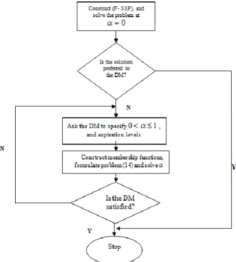
6. Solution procedure

In this section, an interactive solution procedure for solving the (F- SSP) is introduced as

Step1:Construct the (F- SSP).

Step2: At





0

, calculate the individual minimum and maximum of each objective function withrespect to the given constraints, if the solutions preferred to the DM go to step6. Otherwise go to step3.

Step 3: Ask the DM to select the initial value of



(

0







1

),

and the aspiration levels.

Step 4: Elicit the membership functions,



_k

(

f

k

),

k



1

,

2

,

3

.

Step 5: Formulate the problem (11), and problem (14), and solve it to obtain



-optimal compromise solution. If the DM satisfied with the solution, go to step6. Otherwise, go to step3.

[image:7.595.180.421.54.321.2]

Fig.1. Flowchart for the solution procedure

7. Numerical example

Consider the (F- SSP) as

    

  

 



_{ }

_{ }

_{ }

 

 

 

ij

i j

ij ij

i j

ij ij

i j

ijx f x q q x f x l l x

p p

x f

4

1 5

1 3

4

1 5

1 2

4

1 5

1 1

~ )

~ , ( ~ , ~ )

~ , ( ~ , ~ )

~ , ( ~ min

Subject to

integer.

and

,

5

...

,

1

;

4

...,

,

1

,

0

;

~

~

;

4

...,

,

1

,

~

4

1 5

1 5

1













_



  

j

i

x

B

x

p

i

C

x

_{ij ij}

i j ij i

j ij

Fuzzy demands for the items are: 2000 =(1300, 1500, 2000, 2200), 5000=(3500, 4500, 5000,6000), 3000= (2000, 2500, 3000, 3500), 4000=(3000, 3500, 4000, 4500), and 2000=(1000, 1500, 2000, 2500).

Fuzzy capacities are 550= (400, 500, 550, 600), 5000=(3500, 4500, 5000,5500), 2450=(2000, 2200,2450, 2600), and 8000= (6000, 7000, 8000, 10000)

Fuzzy allocated budget is 200000= (100000, 150000, 200000, 250000).

[image:7.595.35.567.572.703.2]

The fuzzy data can be represented as trapezoidal fuzzy numbers as in the following table

Table 1. Trapezoidal fuzzy data related to the multi- item / multi- supplier problem

Item1 Item2 Item3 Item4 Item5

Supplier1

Price (2,4,5,6) (5,8,9,11) (1,2,3,5) (4,6,7,9) (1,2,3,5)

Rejected rate (.01, .02, .03, .04) (.01,.03,.04,.05) (0, .01, .02, .03) (.01, .02, .03, .04) (.01, .02, .03, .04) Late delivery (.02, .04, .0.05, .06) (0, .01, .02, .03) (0, .01, .02, .03) (.02, .04, .0.5, .06) (.01, .02, .03, .04)

Supplier2

Price (3, 5, 6, 7) (4,6,7,9) (1, 3, 4,5) (2,4,5,6) (1,2,3,5)

Rejected rate (0, .01, .02, .03) (.01,.03,.04,.05) (0, .01, .02, .03) (0, .01, .02, .03) (.01, .02, .03, .04) Late delivery (.01,.03,.04,.05) (.01, .02, .03,.04) (.01, .02, .03,.04) (0, .01, .02, .03) (0, .01, .02, .03)

Supplier3

Price (1,2,3,5) (5,8,9,11) (1,2,3,5) (3, 5, 6, 7) (1,2,3,5)

Rejected rate (.01,.03,.04,.05) (.01,.03,.04,.05) (.01, .02, .03,.04) (.01, .02, .03,.04) (0, .01, .02, .03) Late delivery (.01,.03,.04,.05) (.02, .04, .0.05, .06) (0, .01, .02, .03) (.01, .02, .03,.04) (0, .01, .02, .03)

Supplier4

Price (1, 3, 4,5) (6,9,10,11) (1,2,3,5) (3, 5, 6, 7) (1,2,3,5)

Rejected rate (.01,.03, .04, .05) (0, .01, .02, .03) (0, .01, .02, .03) (.01,.03,.04,.05) (.01, .02, .03,.04) Late delivery (.01,.03, .04, .05) (.01,.03,.04,.05) (0, .01, .02, .03) (.01,.03,.04,.05) (.01, .02, .03,.04) Let us apply the steps of the solution procedure as:

Step2: The individual maximum and minimum are:

 

Z

1 max



93600

,

 

Z

1 min



78000

,

 

Z

2 max



275

,

 

Z

2 min



220

,

 

Z

3 max



290

,

 

Z

3 min



200

.

[image:8.595.35.559.69.201.2]

Table 2. Interval of confidence corresponding to fuzzy data related to the multi- item / multi- supplier problem

Item1 Item2 Item3 Item4 Item5

Supplier1

Price [3.4, 5.3] [7.1, 9.6] [1.7, 3.6] [5.4, 7.6] [1.7, 3.6]

Rejected rate [.017, .033] [.024, .043] [007, .037] [.017, .033] [.017, .033] Late delivery [.034, .067] [007, .037] ([007, .037] [.034, .067] [.017, .033]

Supplier2

Price [4.4, 6.3] [5.4, 7.6] [2.4, 4.3] [3.4, 5.3] [2.4, 4.3]

Rejected rate [.007, .023] [.017, .037] [.017, .037] [.007, .023] [.017, .033] Late delivery [.017, .037] [.017, .033] [.017, .033] [.007, .023] [.007, .023]

Supplier3

Price [1.7, 3.6] [7.1, 9.6] [1.7, 3.6] [4.4, 6.3] [1.7, 3.6]

Rejected rate [.017, .037] [.017, .037] [.017, .033] [.017, .033] [.007, .023] Late delivery [.017, .037] [.034, .053] [.017, .037] [.017, .033] [.007, .023]

Supplier4

Price [2.4, 4.3] [8.1, 10.3] [1.7, 3.6] [4.4, 6.3] [1.7, 3.6]

Rejected rate [.017, .037] [.007, .023] [.007, .023] [.017, .037] [.017, .033] Late delivery [.017, .037] [.017, .037] [.007, .023] [.007, .023] [.007, .023]

], 4150 , 3350 [ ], 3150 , 2350 [ ], 5300 , 4200 [ ], 2060 , 1440

[ _{2 3 4}

1 D  D  D 

D D₅[1350,2150],

] 8600 , 6700 [ ], 2495 , 2140 [ ], 5150 , 4200 [ ], 565 , 470

[ _{2 3 4}

1 C  C  C 

C , and

B



[

135000

,

215000

].

Step5: Formulate the problem according to problem (14)

[image:9.595.77.519.360.566.2]

0 , , , , , ; 5 , 4 , 3 , 2 , 1 ; 4 , 3 , 2 , 1 ), (int 0 , 1 0 , 220 023 . 0 023 . 0 023 . 0 037 . 0 037 . 0 023 . 0 033 . 0 037 . 0 053 . 0 037 . 0 023 . 0 023 . 0 033 . 0 033 . 0 037 . 0 033 . 0 067 . 0 037 . 0 037 . 0 067 . 0 , 275 033 . 0 037 . 0 023 . 0 023 . 0 037 . 0 023 . 0 033 . 0 033 . 0 037 . 0 037 . 0 033 . 0 023 . 0 037 . 0 037 . 0 023 . 0 032 . 0 033 . 0 037 . 0 043 . 0 033 . 0 , 93600 6 . 3 3 . 6 6 . 3 3 . 10 3 . 4 6 . 3 3 . 6 6 . 3 6 . 9 6 . 3 3 . 4 3 . 5 3 . 4 6 . 7 3 . 6 6 . 3 6 . 7 6 . 3 6 . 9 3 . 5 3 2 1 3 2 1 3 3 45 44 43 42 41 35 34 33 32 31 25 24 23 22 21 15 14 13 12 11 2 2 45 44 43 42 41 35 34 33 32 31 25 24 23 22 21 15 14 13 12 11 1 1 45 44 43 42 41 35 34 33 32 31 25 24 23 22 21 15 14 13 12 11                                                                                                                                       d d d d d d j i egers x d d x x x x x x x x x x x x x x x x x x x x d d x x x x x x x x x x x x x x x x x x x x d d x x x x x x x x x x x x x x x x x x x x ij 

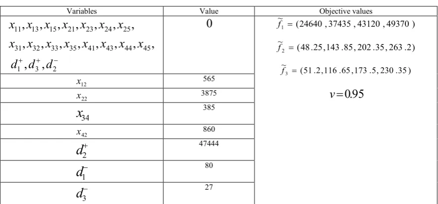
Table 3. The Efficient fuzzy solution

Variables Value Objective values

   2 3 1 45 44 43 41 35 33 32 31 25 24 23 21 15 13 11

,

,

,

,

,

,

,

,

,

,

,

,

,

,

,

,

,

d

d

d

x

x

x

x

x

x

x

x

x

x

x

x

x

x

x

0

~f1 (24640,37435,43120,49370)

) 2 . 263 , 35 . 202 , 85 . 143 , 25 . 48 ( ~ 2  f ) 35 . 230 , 5 . 173 , 65 . 116 , 2 . 51 ( ~ 3  f

95

.

0



v

12 x 565 22 x 3875 34

x

385 42 x 860  2

d

47444  1

d

80  3

d

27

8. Concluding remarks

In this paper, multiple sourcing supplier selection (F-SSP) problem was introduced as multi- objective linear programming problem with fuzzy parameters represented as trapezoidal fuzzy numbers. An interactive fuzzy goal programming approach has been applied to provide the



- best compromise solution for the (



-SSP) problem. This approach helps the DM to select the better supplier in the supply chain.

Acknowledgements

The authors are very grateful to the anonymous reviewers for his/ her insightful and constructive comments and suggestions that have led to an improved version of this paper.

REFERENCES

Agakishiyev, E. 2016. Supplier selection problem under Z- information. Procedia Computer Science, (102): 418-425.

Amid, A., Ghodsypour, S.H., and O' Brien, C. 2006.Fuzzy multiobjective linear model for supplier selection in a supply chain.

International Journal of Production Economics, (104): 394- 407.

Arikan, F. 2013. An interactive solution approach for multiple objective supplier selection problem with fuzzy parameters. J.

Bellman, R., and Zadeh, L. A. 1970. Decision making in a fuzzy environment. Management Science, (17): 141-164.

Biswal, M. P. 1992. Fuzzy programming technique to solve multiobjective geometric programming problems. Fuzzy Sets and

Systems, (51): 67-71.

Chan, F. T. S., and Kumar, N. 2007. Global supplier development considering risk factors using fuzzy extended AHP- based approach. The International Journal of Management Science, (35) 417- 431.

Davari, S., Zarandi, M. H.F., and Turksen, I.B.2008. Supplier selection in a multi- item/ multi- supplier environment. Fuzzy Information Processing Society. Annual Meeting of the North American.

Diaz-Medronero, D. M., Peidro, D., and Vasant, P. 2010. Vendor selection problem by using an interactive fuzzy multiobjective approach with modified S-curve membership functions. Computers and Mathematics with Applications, 60(4): 1038-1048. Dubois, D., and Prade, H. 1980. Fuzzy Sets and Systems: Theory and Applications. Academic Press, New York.

Ekhtiari, M., Poursafary, S. 2013. Multi-objective stochastic programming for mixed integer vendor selection problem using artificial bee colony algorithm.Artificial Intelligence, Article ID795752, 13 pages.

He, S., Chaudhry, S. S., Lei, Z., and Baohua, W. (2009). Stochastic vendor selection problem; chance-constrained model and genetic algorithms. Annals of Operations Research, (168): 169-179.

He, X., and Zhang, J. 2018. Supplier selection study under the respective of the low- carbon supply chain: a hybrid evaluation model based on FA- DEA- AHP. Sustainability, 10, 564; doi: 10.3390/ su10020564.

Kaufmann, A., and Gupta, M. M. 1988. Fuzzy Mathematical Models in Engineering and Management Science. Elsevier Science Publishing Company INC, New York.

Khalifa, A.H. 2017. Interactive fuzzy programming approach for vender selection problem in supply chain with fuzzy parameters.

Fuzzy Mathematics, 25(4): 239-250..

Kumar, J., and Roy, N. 2010. A hybrid method for vendor selection using neural network. International Journal of Computer

Applications, (11): 35-40.

Kumar, M., Vrat, P., and Shankar, R. 2004. A fuzzy goal programming approach for vendor selection problem in a supply chain.

Computers& Industrial Engineering, 46(1): 69- 85.

Kumar, M., Vrat, P., and Shankar, R. 2006, A fuzzy programming approach for vendor selection problem in a supply chain.

International Journal of production Economics, (101): 273-285.

Mendoza, A., Santiago, E., and Ravindron, R. A. 2008. A three-phase multi-criteria method to the supplier selection problem.

International Journal of Industrial Engineering, 5 (2): 195-2120.

Moore, E. R., 1979. Methods and applications of interval analysis (SIAM, Philadephia, PA).

Narasimhan, R., and Talluri, S. 2009. Perspective on risk management in supply chains. Journal of Operations Management,27 (2): 104-114.

Pan, A. C. 1989. Allocation or order quantity among suppliers. Journal of Purchasing and Material Management, (10): 36-39. Polat, G., Eray, E.,NevalBingol, B. 2017. An integrated fuzzy MCGDM approach for supplier selection problem. Journal of Civil

Engineering and Management, 23(7):926-942.

Sakawa, M. 1993. Fuzzy Sets and Interactive Multiobjective Optimization. New York, USA: Plenium Press.

Sakawa, M., and Yano, H. 1989. Interactive decision making of multi-objective nonlinear programming problems with fuzzy Parameters. Fuzzy Sets and Systems, (29): 315-326.

Scott, J., and Talluri, S. 2015. A decision support system for supplier selection and order allocation in stochastic, multi- stakeholder and multi-criteria environments. International Journal of Production and Economics, (166):226- 237.

Ware, R. N., Sing, P. S., and Bonwet, K. D. 2012. Supplier selection problem: A state-of-the-art review. Management Science

Letters, (2): 1465-1490.

Weber, C.A., and Current, J. R. 1993. A multi- objective approach to vendor selection. European Journal of Operations Research,

(68): 173- 184.

Xia, W., and Wu, Z. 2007. Supplier selection with multiple criteria in volume discount environments. Omega the international

Journal of Management Science, (35): 494- 504.

Zhou, Z., Dou, Y., Liao, T., and Tan, Y. 2018. A preference model for supplier selection based on hesitant fuzzy sets. with several objective functions. Sustainability, 10, 659; doi: 10.3390/ su10030659.

Zimmermann, J. H. 1978. Fuzzy programming and linear programming with several objective functions. Fuzzy Sets and Systems,

(1): 45- 55.