GENETIC NETWORK PROGRAMMING REINFORCEMENT LEARNING BASED SAFE AND SMOOTH MOBILE ROBOT NAVIGATION IN UNKNOWN DYNAMIC ENVIRONMENTS

GENETIC NETWORK PROGRAMMING-REINFORCEMENT

LEARNING BASED SAFE AND SMOOTH MOBILE ROBOT

NAVIGATION IN UNKNOWN DYNAMIC ENVIRONMENTS

1,2

AHMED H. M. FINDI, 3MOHAMMAD H. MARHABAN, 4RAJA KAMIL, 5MOHD KHAIR

HASSAN 1

Department of Electrical and Electronic Engineering, Faculty of Engineering, Universiti Putra Malaysia, Malaysia.

2

Control and Systems Engineering Department, University of Technology, Baghdad, Iraq. 3

Prof, 4, 5 Assoc. Prof. Department of Electrical and Electronic Engineering, Faculty of Engineering,

Universiti Putra Malaysia, Malaysia.

E-mail: 1ahmfindi@gmail.com, 3mhm@upm.edu.my, 4kamil@eng.upm.edu.my, 5khair@eng.upm.edu.my

ABSTRACT

The problem of determining a smoothest and collision-free path with maximum possible speed for a Mobile Robot (R) which is chasing a moving target in an unknown dynamic environment is addressed in this paper. Genetic Network Programming with Reinforcement Learning (GNP-RL) has several important features over other evolutionary algorithms such as combining offline and online learning on the one hand, and combining diversified and intensified search on the other hand. However, it was used in solving the problem of R navigation in static environment only. This paper presents GNP-RL as a first attempt to apply it for R navigation in dynamic environment. The GNP-RL is designed based on an environment representation called Obstacle-Target Correlation (OTC). The combination between features of OTC and that of GNP-RL provides safe navigation (effective obstacle avoidance) in dynamic environment, smooth movement, and reducing the obstacle avoidance latency time. Simulation in dynamic environment is used to evaluate the performance of collision prediction based GNP-RL compared with that of two state-of-the art navigation approaches, namely, Q-learning (QL) and Artificial Potential Field (APF). The simulation results show that the proposed GNP-RL outperforms both QL and APF in terms of smoothness movement and safer navigation. In addition, it outperforms APF in terms of preserving maximum possible speed during obstacle avoidance.

Keywords: Genetic Network Programming with Reinforcement Learning (GNP-RL), Mobile robot

navigation, Obstacle avoidance, Unknown dynamic environment

1. INTRODUCTION

Nowadays, navigation in dynamic environment is one of the emerging applications in mobile robot (R) field. The research on navigation in static environment is already matured [1], however, in dynamic environment, which is crucial for many real world applications, has recently received substantial attention [2, 3]. The goals of navigation are obstacle avoidance and navigation time reduction. Nevertheless, another important feature that should be included during navigation is minimizing robot steering angle during obstacle avoidance while providing maximum possible speed to preserve R smooth movement and to avoid big changes in speed set point.

static and predefined. On the other hand, machine learning algorithms [16-18] were proposed to obtain time-optimal and collision free path of a R during its navigation in dynamic environment. However, a precise input/output dataset should be provided for training process of these algorithms, but obtaining the dataset is hard or sometimes is impossible [19]. Instead, reinforcement learning techniques [8, 20] are used to learn robots by its online interaction with the environment without the need to provide a dataset.

Artificial Potential Field (APF) [6, 16, 21-26] is one of the most commonly used schemes in the field of R navigation [20]. In the work of Ge and Cui [22], the authors applied APF in a dynamic environment containing a moving target where the movement of R is assumed to be affected by two potential field forces. The first field is called the attractive potential field, which is generated by the target and produced an attractive force that attracts R to the position of the target all the time. The second field is called repulsive potential field, which is generated by the obstacles and produced a repulsive force that moves R away from these obstacles. Consequently, R moves under the effect of the sum of these two forces where the repulsive force is calculated as the sum of all repulsive forces generated by all the obstacles in the environment. However, APF suffers from local minima problem [16]. In addition, preserving the smoothest path during obstacle avoidance has not been considered in these works.

In 2001, Mucientes et al. [27] presented Temporal Fuzzy Rules (TFR) to provide avoidance of collision even when the moving obstacles behave in a totally unexpected manner. The works in [2, 28, 29] presented virtual plane, generalized velocity obstacle, and reactive control design, respectively, to allow R to avoid dynamic obstacles. However all these techniques are based on measuring the velocity of moving obstacles. Practically, this measurement is noisy and difficult to obtain [28, 30] .

In 2011, Jaradat et al. [20] presented a smart definition of the environment states to represent an unknown dynamic environment with a moving target to utilize Q-learning with a finite number of states. However, the smooth movement and speed control of R are not considered in their work, where

R should turn strictly (

±

π

/

4

with an obstacle and it always moves with constant speed even if there is no obstacle in its way. Hereinafter, this methodology is referred as

Obstacle Target Correlation based Q-Learning (OTCQL).

GNP-RL [31-36] is an extension of GNP [37] and it is efficiently combined evolution and learning.

Evolutionary computation generally has an

advantage in diversified search ability, while reinforcement learning has an advantage in intensified search ability and online learning. Up to our knowledge, GNP-RL designs have been used in solving the problem of R navigation in static environment only and based on sensor readings as inputs which are efficient in static environment. However, in dynamic environment, sensor readings provide infinite number of states to cover all variations of dynamic environment. Therefore, it requires inflation in GNP-RL nodes to cover all

these states. Hence, providing environment

representation that represents all states of environment in definite number of states is necessary.

This paper presents an attempt to apply GNP-RL to control navigation of R in dynamic environment. A novel GNP-RL design is presented based on the incorporation of the parameters of an environment representation, called Obstacle-Target Correlation (OTC), into the judgment nodes of GNP-RL. This proposed design aims to obtain effective obstacle avoidance using minimum change in steering angle between the consecutive steps to smooth path trajectory of R and finding maximum possible speed that is sufficient to exceed obstacle successfully without enforcing a high slowness on robot speed. The main objectives of this paper are:

• Safe navigation in dynamic environment

containing a combination of static and dynamic obstacles during chasing a moving target.

• Finding the minimum steering angle changes

between consecutive steps of R during obstacle avoidance in such a way that R can move smoothly without using sharp turning.

• Control the speed of R during obstacle avoidance

to compromise between maintaining the

maximum possible speed and providing safe path.

• Integrating OTC and GNP-RL to earn the

benefits of both conceiving the surrounding environment and features of GNP-RL and to

apply it for R navigation in dynamic

2. THE ENVIRONMENT REPRESENTATION

The objective of this section is to represent unknown dynamic environment surrounding R at any instant of navigation process by a number of variables. These variables give a considerable perception of the surrounding environment in such a way that R can navigate safely without colliding with any obstacle until catching a moving target. Fig.1 shows the representation of an environment that surrounds R.

2.1. Definitions and Assumptions

The following definitions and assumptions are made [20].

1. The position of , at each instant refers

to the origin of the coordination and its goal is

catching the target , . While, G is

continuously moving and its instantaneous coordinates are known to R throughout all the time of navigation without knowing its future trajectory.

2. The environment is unknown and it contains many obstacles which are either static or

dynamic. The dynamic obstacles ( ) are moved

randomly and behaved in a totally unexpected manner. At each time instant, R deals with one obstacle and the nearest obstacle to R is denoted

by , .

3. The robot has a sensory system which is used to measure the real time position of the obstacles in a specific range.

4. The speed of R is always greater than that of G,

i.e. , and it is always greater than or

equal to that of obstacles i.e. .

5. R becomes in non-safe mode if

otherwise, it is in safe mode. Collision happens

between R and when . On the other

hand, R is considered catching G if ,

where is the distance between Rand ,

is a safety distance, is the collision

distance, is the distance between R and G,

and is the winning distance.

Fig.1 The Environment Representation. (A) Analysis Of Target And Obstacle Positions Related To R Position (B)

Divisions Of The Angle Α.[20] 2.2. The Environment Model

The environment model presented in [20] is considered in this paper. As shown in Fig.1, the environment of the robot consists of its target and an obstacle. The target is dynamic and the obstacles may be static or dynamic. The environment around R is divided into either four orthogonal

regions: 1 4or eight regions . At

each instant, the environment is represented by the

region that contains the target , the region that

contains the closest obstacle to the robot ( ) and

the region of the angle between the robot to

obstacle line and the robot to target line ( ,

where the angle is computed as in eq.1:

1

sin

RO

D

d

α

where D is the distance between the obstacle and R

to target line. and are found in one of the

orthogonal regions: 1 4, while is found in

one of the eight regions as shown in

Fig.1.

3. THE PROPOSED GNP-RL

successfully without need to excessive slowness of robot speed.

3.1. GNP-RL Structure

GNP-RL is constructed of several nodes (n) connected with each other and each node has a unique number (0 to n-1). These nodes are classified into start node, judgment node, and processing node as shown in Fig. 2. The judgment nodes and processing nodes are interconnected to each other by directed links that indicate the possible transitions from one node to another. The starting node has neither function to do nor conditional outbound connections. But it represents the starting point of each node transition and it functions to determine the first node, judgment or processing, in node transition to be executed in GNP-RL. Therefore, the first node is determined by the outbound of the starting node which has no inbound connection. Every judgment node has many outbound connections, so one of these connections is selected according to if-then decision functions to find the next node to be executed. While the processing nodes, which are responsible for providing the suitable actions of R, have only one outbound connection corresponding to each action. On the other hand, judgment and

processing operations require time to be

implemented. This time is called time delay ( ), which is assigned to each node, and participated in evolving flexible and deadlock free programs.

Fig. 2. Basic Structure Of GNP-RL [31] The gene structure of each node is divided into two parts; macro node and sub-node parts as shown in Fig. 3. The macro part consists of node type (!") and time delay spent on executing a node ( ),

where

i

!"is set to 0, 1, or 2 to refer to start, judgment or

processing nodes, respectively. of judgment

nodes is set to one time unit and that of processing nodes is set to five time units. The sub-node part consists of the judgment/processing code number

(#$%) which is a unique number, value of judgment

(&_%), value of processing ('_%(), Q value ()_%() and

the next node numbers connected from sub-node k in node

i

sub-node,in the node +, 1 , ., and . is the

number of sub-nodes in node +.

In this work, #$%represents the region, , ,or

to be judged by judgment nodes and direction of turning, left or right, for processing nodes, while &_%

represents the value of judgment which contains the region value of target, obstacle or angle. Since

and take one of four values and takes one of

eight values, then either four or eight Q-values can be found in every sub-node of judgment nodes

depending on the parameters ( , ,and ) of

#$_%. Similarly, there are either four or eight *_%(in

each sub-node of judgment nodes. For processing

nodes, '%( refers to angle of turn and robot speed

for -=1 or 2, respectively. In addition, there is only

one Q-value and one *%(in each sub-node and .

is set to 2 for both judgment and processing nodes.

The proposed GNP-RL contains one starting node, 16 judgment nodes and 10 processing nodes. Once R encounters an obstacle, the controller turns from safe mode to non-safe mode in which GNP-RL guides R by starting the node transition. This transition aims to find a suitable processing action through judging current environment state.

The node transition embarks with the start node which guides the execution to one of the judgment

or processing nodes. If the current node

i

judgment node, one of the )%(in each sub-node is

selected based on the corresponding values of

#$_%and &_%. The maximum Q-value among the

selected Q-values is chosen with the probability

1 / or random one is chosen with the probability

of /. Then the corresponding *%(is selected. If the

current node is processing, maximum of ) and

)0 is selected when the probability is 1 /, but

one of these Q-values is chosen randomly when the

probability is /. Corresponding to the selected

Q-value, the values of the #$%, '% ,'%0, *% specify

robot movement direction, left or right, the degree of robot turning angle, the speed of the robot, and the number of the next node, respectively.

turning angle and speed to avoid the encountered obstacle. Moreover, the selected processing node specifies the next node in GNP-RL, which should be executed if the non-safe state still valid. This process continues until R avoids the encountered obstacle and changes from non-safe to safe state.

Fig. 3. The Gene Structure Of GNP-RL Nodes

3.2. Learning and Evolution Process

The learning aims to train individuals to find the best node transition of each one by updating the Q-values through State Action Reward State Action

(SARSA) [38], while evolution process aims to find

the best structure of GNP-RL in population by evolving individuals along all generations. As shown in Fig. 4, the first step of learning and evolution process is the initialization of population in which the parameters and values of connections and node functions are set randomly while all Q-values are set to zero. The second step is applying all learning trials on each individual to update its Q-values and measure its fitness. At the end of each generation, the individual with the highest fitness is chosen as an elite individual and passed directly to the population of the next generation without any modification. The complementary individuals of the next generation are obtained from applying genetic operations: selection, crossover and mutation. At the last generation, the individual that provides best performance among all individuals is chosen to be utilized in controlling R in the testing task.

3.2.1. Q- values update using SARSA

The node transition of GNP-RL starts once the robot encounters an obstacle and it continues until obstacle avoidance takes place. The flowchart in Figure 4 illustrates the node transition in judgment and processing nodes. The Q-values updating is fulfilled as follows:

1- Suppose the current node is judgment

i

Then one of the )%( in each sub-node is

selected based on the corresponding values of

#$% and &%. The maximum Q-value among the

selected Q-values is chosen with the probability

of 1 / or random one is chosen with the

probability of /.

2- The selected Q-value refers to the selected

sub-node. Hence, the corresponding *%(can be

identified, which, in turn, refers to the next node.

3- The node transition is transferred from current

node + to next node 1 and one )%(is selected by

the same way shown in step 1.

4- Repeat steps 1, 2 and 3 until *_%(refers to a

processing node.

5- When the next node 1 in node transition is a

processing node, maximum of ) and )0 is

selected when the probability is1 /, but one of

these Q-values is chosen randomly when the

probability is /. Corresponding to the selected

Q-value, the values of R movement direction (left or right) (#$% , the degree of R turning

angle ('% ), the speed of R ('%0), and the

number of the next node (*_% ) are specified.

6- Judge the robot movement related to the

obstacle and get reward 23.

7- The Q-values update in Equation 2 is based on

SARSA learning and carried out on all nodes along the node transition.

( )

: ( 0 1)

: ( 0 1)

i

ik p k p t jk p ik p

Q Q r Q Q

le arn in g rate

d is c o u n t rate

η

µ

η

η

µ

µ

← + + −

< ≤

< ≤

(2)

3.2.2. Genetic operations

Crossover is executed between two parents generating two offspring. The first step of executing crossover operation is selecting each

node

i

using tournament selection, as a crossover node

with the probability of Pc. Then, the two parents swap the genes of the corresponding crossover nodes (i.e. with the same node number). As a result, the generated offspring become the new individuals in the next generation.

On the other hand, mutation is executed in one individual and a new individual is generated. The first step of executing mutation operation is selecting one individual using tournament selection. Then with the probability of Pm, each node branch is re-connected to another node, each node function (region type in the case of judgment and right/left turning in the case of processing) is changed to

another one, and each parameter '_%( in the

processing node is changed to another value. Finally, the generated new individual becomes the new one in the next generation.[31].

3.2.3. Fitness Function

In a dynamic environment with a moving target, R tries to navigate safely from a start location to a location of catching the moving target. During this navigation, R should find a feasible collision-free path in which the steering angle changes between consecutive steps should be as less as possible and the movement should be fast enough to exceed obstacle without collision. The fitness function is designed to satisfy this purpose.

During the learning task, every individual in a population in each generation has to fulfill obstacle avoidance during target chasing in every trial. A trial ends when R catches G, obstacle collision takes place, or the time step reaches the predefined time step limit (=100). At every step throughout

obstacle avoidance activity, the reward (23)

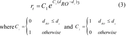
obtained by R is calculated by Eq. 3. The reward function is ranged between [0 1] and designed in order to learn obstacle avoidance behavior, that is,

R has to avoid obstacles with trying to make as

large as possible where the reward decreases when R closes to an obstacle and vise versa.

2( )3

1

s

C d d

t

RO

r

=

C

e

where 1

{

0

1

RO c

d d

C

otherwise

≤

= _and

{

2

1

0

RO s

d d

C

otherwise

≤ =

The fitness function is designed to measure the performance of R according to its steering angle change and speed. Hence, the fitness function of GNP-RL takes into account both objectives: minimization of steering angle change and

avoidance. The fitness function is calculated by Eq.4 when all trials of an individual end.

2 2 max 1 1 3 ( ) ( ) 1 R N M n m t

r v v

fitness N M

C r

e

ϖ

=

∑ ∑

where N is the total number of trials, M is the

number of steps required to avoid an obstacle,

max max

1

( ) T T

r θ θ θ θ

θ θ

−

− ∆

∆ = = is the rate of steering

angle change (∆5) between two consecutive steps,

is the speed of the R, 678 is the maximum

speed of the R, ₃

{

5 RO d _dc C otherwise ≤ = ,and

total right left

total

η η η

ϖ

η

− −

= _{is a factor of balancing the}

movement of R in both directions where ηtotal,

right

η , and ηleft are the total turning actions,

number of turning to the right, and number of turning to the left during obstacle avoidance in all trials of an individual, respectively. This factor is used to prevent R from tending to move in one direction to minimize steering angle on the account of safe navigation.

Fig. 5 shows the distribution of the fitness function values when its parameters are changed along all

their range where it is assumed that 9 1.5.,

9 0.3., and 9 2.. It can be noted that the

fitness values are increased when steering angle change is decreased and speed is increased. That is, the fitness values go to their maximum value when steering angle change approaches to zero and speed approaches to its maximum value.

Fig. 5 Fitness Function

3.3. Target Tracking

In every learning or execution experiment, R embarks from its starting point and it continuously adjusts its orientation towards G. the speed of R is set to maximum value when its path is free of

obstacles (safe mode) and it adjusts its steering angle towards G according to Eq.5

max

max

( 1) * cos( ( ))

( )

( ) ( 1) * sin( ( ))

x RG

x

y y RG

R T v T

R T

R T R T v T

θ θ − + = − +



















 



where θ_RG( )T is the angle measured at instant T of

the virtual line connecting R and G. But GNP-RL controls R speed and steering angle when it faces an obstacle (non-safe mode) according to Eq. 6

where the speed of R is set byA_ik2 and θ_{R G}( )T is

either increased or decreased byA_ik1 depending on

the direction of turning which is set byID_ik .

2 1

2 1

( ) ( 1) * cos( ( ) )

( ) ( 1) * sin( ( ) )

x x ik ik

y y ik RG ik

RG

R T R T A T A

R T R T A T A

θ θ − + = − +



 





 





 



3.4. GNP-RL Setup

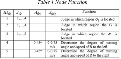
As shown in Table 1, there are sixteen judgment

functions and two processing functions because ,

,and have sixteen states and R should turn to

either left or right to avoid the encountered obstacle. Each processing node sets the degree of

turning and speed of R at '_% and '_%0

respectively.

Table 1 Node Function

The evolution and learning parameters are shown in Table 2. The number of initial population,

crossover probability, mutation probability,

tournament size, and maximal offspring generation are set by 400, 0.1, 0.01, 6, and 6000, respectively, while the parameters of learning process are set by

B 9 0.9, D 9 0.3, and / 9 0.1.The population in

randomly based on their valid ranges, while the Q values of the sub-nodes are set to zero. The sum of

i

d _{of all nodes used in a node transition of one R}

step should not exceed 21 time unites. If it exceeds this predefined time units without executing a processing node, R takes the same action in the previous step. Hence, the maximum number of nodes that can be used in one node transition cycle is sixteen judgment nodes and one processing node. As a consequence, this process prevents node transition from falling in non-stop loops

Table 2 Simulation Parameters

4. SIMULATION

The simulation is composed of two tasks: learning and execution. The learning task aims to find an individual that has the ability to achieve the desired safe, smooth, and fast navigation. The selected individual in the learning phase is tested in the execution phase throughout exposing R to intensive and complicated experiments. In this paper, the simulation is implemented using MATLAB software.

4.1. Learning Task

The individual that has the best performance is found during the learning task. On one hand, the learning task produces an individual from search space that has the connections which can provide the best performance of R. On the other hand, SARSA is used to learn each individual in such a way that a connection in a judgment node among all available connections or an action in a processing node among all available actions is selected for each surrounding environment state.

In GNP-RL, an individual represents a network of GNP-RL. The performance of a GNP-RL is evaluated as follows. R moves from the start point and chases the moving target in every trial. A 100

trails,

N

=

100

contains a static and a dynamic obstacles. The GNP-RL is applied to control R when it is in non-safe mode. The rate of steering angle change,

2 Δ5 , and the set point of speed ( ) are used in

calculating the fitness value in each step of non-safe mode. After applying GNP-RL on all trials, the

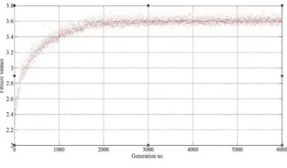
fitness value of that individual is calculated using Eq.4. These steps are repeated on all individuals in the population. The individual with highest fitness is selected as elite. The genetic operations, selection, crossover, and mutation, are then applied to generate the next generation. Since then, the same steps of calculating the fitness values are applied to each individual to find the individual that has the highest fitness. In this paper, the total number of generations is 6000, and the highest fitness value in each generation is shown in Fig. 6. It can be seen that the highest fitness value of the first generation is 2.063, and this value is continuously changed along all generations until it stabilizes at 3.614 in the last generation. The individual which has the highest fitness value (elite) in the last generation is used later in the execution task to measure its efficiency in providing the required safe navigation and smooth movement.

Fig. 6. Fitness Values Of GNP-RL

4.2. Execution Task

After accomplishing the learning task, which

produces a GNP-RL network with best

performance among all other networks in the search space, several test scenarios were conducted to assess the performance of GNP-RL under wide variety of environment conditions in which several static and dynamic obstacles were used to disturb the R movement.

4.2.1. Execution test

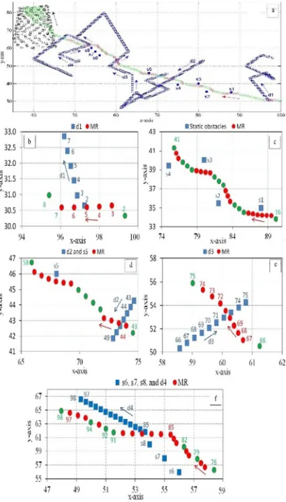
Many experiments were conducted to test the efficiency of the proposed GNP-RL. One of these experiments is explained in this section as shown in Fig.7. In this experiment, four dynamic obstacles (d1-d4) that move randomly and eight static obstacles (s1-s8) are located in the work space. In addition, the dynamic target (black color) is moving in upward exponentially sinusoidal form starting

0.02 ( 90 )

3 * sin 0.3

0.15

y

G y

x

G y

G v

v

v

e− −

= =









 

_





_





 

_

_

 





The movements and locations of R, dynamic obstacles, static obstacles, and G are shown in Fig.

7(a). The set point of is set to maximum (0.75

m/s) when it is in safe mode (green color) F

. But when R becomes in the non-safe mode (red color), this set point is controlled by GNP-RL, while the speed of each dynamic obstacle (d1-d4) is 0.5 m/s. Fig. 7(b-f) are expansions of the environment in obstacle avoidance occurrences to illustrate the details of R steps at those moments. In

this scenario 9 0.3., 9 2., and 9

0.3..

R started its navigation at [100 30]T with maximum

speed to chase G and adjusted its turning angle towards the target but it encountered d1 at [98.65 30.66]T when it was in the third step as shown in Fig. 7(b) . At this moment the robot controller was changed from safe to non-safe mode in which GNP-RL changed the steering angle of R to the left

by (28.92˚) and changed the set point of speed to

0.65 m/s. The steering angle changes (∆5) in all the

consecutive steps are almost close to zero without change in speed. This action helped R to exceed d1

successfully, where minimum 9 1.55., with

smooth path and satisfactory speed.

Fig. 7(c) shows the capability of R under control of GNP-RL to exceed static obstacles. In step 17, R encountered s1 that made it changes its movement to the left for six steps to be in safe mode and continued its way to the target. Later, s2, s3, and s4 were also exceeded until it became in safe mode in

step 41 where the maximum ∆5 used in static

obstacles avoidance is 30.38˚.

Fig. 7(d) and (e) show the effect of GNP-RL on R response when it faced two dynamic obstacles that disturbed its movement from different directions. In both cases, GNP-RL handles the problem of collision occurrence by changing its direction to the either left or right. No big steering angles have been used to avoid these obstacles where maximum

33.36 θ

∆ = otook place in the first and last steps of

each non-safe region, while small steering angles used in the following steps.

Fig. 7(f) gives an example of disturbing R movement by static obstacles and a dynamic obstacle that is moving in parallel with the

trajectory of R and standing in the way between R and G. In this example, R exceeded s6 and s7 successfully and before completing s8 avoidance it trapped with d4 that is moving in parallel with R. Three tries were done by R to move toward target but it encountered d4 and entered non-safe region. Therefore, GNP-RL moved R away of d4 to avoid this obstacle. This situation made R switches between safe and non-safe regions for three times until R exceeded the effect of d4.

It can be seen that R is capable of avoiding all of static obstacles successfully, though they are located close to each other. It is also noted that the GNP-RL is efficient in avoiding the dynamic obstacles that disturbed R movement from different directions without using sharp turning angles. These obstacles avoidances prove that the robot learned from the experiments in the training phase such that it acquired the capability to avoid this kind of obstacles.

4.2.2. Performance evaluation of GNP-RL

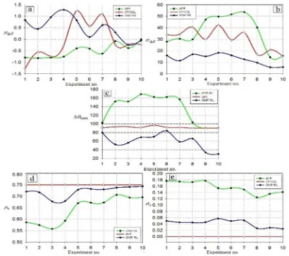
This subsection aims to conduct simulation to examine the efficiency and feasibility of the proposed GNP-RL in comparison with OTCQL [20] and APF [22]. Ten experiments were conducted and applied to each navigation scheme to measure their efficiency under same circumstances. In each experiment, G is moved in either sinusoidal or exponentially sinusoidal form and started its movement from different positions in either direction, different number of dynamic obstacles with random movement, different number of static obstacles, and R started its navigation from different positions. Fig. 8 shows the results of applying these three schemes on the ten experiments.

Referring to Fig 8 (a), it can be noted that the mean

value of steering angle change (D∆G) is ranged

between -1.269 and 1.28 which refers to the

convergence of D∆Gin all schemes under study,

where APF shows the minimum D_∆Gin most of the

conducted experiments. This small range of D∆G is

due to the use of small steering angles during safe mode that are enough to chase the target but the big steering angles are used only during non-safe mode when R encounters an obstacle.

Fig. 8 (b) shows the standard deviation of steering

angle change (H∆G), for all the applied schemes and

it can be seen that GNP-RL shows the minimum

H∆G among all the conducted experiments. That is,

R under control of GNP-RL has the smoothest trajectory path than that of OTCQL and APF where

the difference between H∆Gof GNP-RL and that of

OTCQL is varied between (7.06) and (24.18), and it varied between (8.71) and (41.04) comparing

with APF. Meanwhile, the maximum H∆G in most

of the applied experiments is taken place when R under control of APF which refers to big variations of steering angle producing worst tortuous

trajectory. The maximum angle difference (∆5IJ )

used in every experiment for all the schemes under study proves also this fact. As shown in Fig. 8 (c), the largest steering angles are used by APF to exceed obstacles, while GNP-RL uses the minimum steering angle in all experiments, ranging between (30.06) and (84.07). This refers to the efficiency of GNP-RL to exceed same obstacles with minimum steering angle change. Moreover, OTCQL uses

fixed and large steering angle (m45o_{) during}

obstacle avoidance resulting high H_∆G which refers

to non-smooth navigation path (Fig.8 (a-c)).

However, OTCQL shows moderate ∆5, ranging

around 90˚, between the performance of APF and GNP-RL. Consequently, large steering angles that have been used in APF and OTCQL cause a non-smooth trajectory of R while GNP-RL provides the smoothest path during obstacle avoidance without the need for sharp turning.

According to OTCQL design, the speed of R is constant throughout the entire navigation process (Fig.8 (d-e)). Hence, it is assumed to be set to its maximum value in these experiments. As a result, R under control of OTCQL moves in highest navigation speed than that of other schemes but such R speed control has a negative impact on the efficiency of safe navigation as it will be explained in section 4.2.3. GNP-RL shows its capability to drive R in a reasonable speed ranges between 0.68 and 0.74 m/s while maintaining its smooth

movement. Moreover, GNP-RL shows low

variation of speed (H_K9 0.024, 0.057), that is, R

changes its speed smoothly without the need for sudden changes. In contrast, APF drives R with a

slowest speed (D_K9 0.56, 0.707) and highest

variation of speed (HK9 0.124, 0.177).

Fig. 8. Performance of R under control of GNP-RL, OTCQL, and APF. (a) Mean of ∆N O∆N (b) Standard

deviation of ∆N P∆N (c) Maximum ∆N ∆NQRS (d)

Mean of speed (OT) (e) Standard deviation of speed (PT).

4.2.3. Safe navigation test

This subsection aims to examine the efficiency of the proposed GNP-RL, compared with OTCQL and APF, in exceeding static and dynamic obstacles to satisfy safe navigation.

designed workspace composed of 200 trials; each trial contains 12 dynamic obstacles and 12 static obstacles. The positions of these obstacles are initially predefined and stayed permanent in all trials. The dynamic obstacles are moving in straight lines without changing their directions during the execution time of each trial. But, the orientation angle of all dynamic obstacles is either incremented or decremented in each consecutive trial. Moreover, the movement direction of G and the starting positions of R and G are chosen randomly in each trial, where the movement direction of the target is either up, down, right or left. If any trial in an experiment has no facing between the R and an obstacle, it is repeated with another random selection of positions of R and G until a facing takes place. One of these trials is shown in Fig. 9, which represents the GNP-RL control of R in trial number 143 of one of the conducted experiment. It can be seen that R, which moves to the left, exceeds a dynamic obstacle (d10) and two static obstacles (s2 and s1), respectively, before catching the target which is moving down.

Fig. 9. Workplace Trial Of Dynamic Environment Ten experiments were conducted to measure the degree of safe navigation of R under control of

GNP-RL, OTCQL, and APF where each

experiment includes 200 trials. Hit and miss rates are used as a measure of efficiency of these algorithms. Hit rate can be defined as the frequency of the trials with which R successes to catch G without colliding with any obstacles. Accordingly, the miss rate is the frequency of the trials with which R fails to catch G. Fig. 10 shows the resulting hit/miss rates of applying these ten experiments.

5. CONCLUSION

This paper proposes a new formulation of GNP-RL for R navigation in dynamic environment based on OTC environment representation. R navigation is studied and simulated in an

environment containing static and dynamic

obstacles as well as a moving target. The integration between OTC and GNP-RL provides a suitable action for variant states of the dynamic environment. Efficiency and effectiveness of the proposed GNP-RL have been demonstrated through comparisons with two state-of the arts in R navigation, i.e. OTCQL and APF.

The proposed GNP-RL shows notable improvement in terms of safe navigation, smoothness movement and maximum possible speed to exceed obstacles. For safe navigation, GNP-RL shows approximately

equal performance with OTCQL (GNP-RL

outperforms OTCQL by 1.1% ) and exceeds APF by 4.51%. On the other hand, GNP-RL provides smoothest navigation than that of OTCQL and APF where minimum standard deviation of steering angle of R is presented in all the applied experiments. For fast navigation, R speed is set to maximum when it is under control of OTCQL. Therefore, fastest navigation is shown under such kind of control. However, GNP-RL shows an approximate performance to OTCQL where R speed is near to maximum value with small change in its set point, and it outperforms the speed of APF. In the future, it is recommended to study the effect of replacing the evaluation of the surrounding environment in judgment nodes by fuzzy rules.

REFERENCES:

[1] Zhang, Y., L. Zhang, and X. Zhang. Mobile

Robot path planning base on the hybrid genetic

algorithm in unknown environment. in

Intelligent Systems Design and Applications,

2008. ISDA'08. Eighth International

Conference on. 2008. IEEE.

[2] Belkhouche, F., Reactive path planning in a

dynamic environment. Robotics, IEEE

Transactions on, 2009. 25(4): p. 902-911.

[3] Du Toit, N.E. and J.W. Burdick, Robot motion

planning in dynamic, uncertain environments. Robotics, IEEE Transactions on, 2012. 28(1): p. 101-115.

[4] Parhi, D.R., Navigation of mobile robots using

a fuzzy logic controller. Journal of intelligent and robotic systems, 2005. 42(3): p. 253-273.

[5] Li, W. Fuzzy

logic-basedperception-action'behavior control of a mobile robot in

uncertain environments. in Fuzzy Systems, 1994. IEEE World Congress on Computational Intelligence., Proceedings of the Third IEEE Conference on. 1994. IEEE.

[6] Jaradat, M.A.K., M.H. Garibeh, and E.A.

Feilat, Autonomous mobile robot dynamic

motion planning using hybrid fuzzy potential field. Soft Computing, 2012. 16(1): p. 153-164.

[7] Mobadersany, P., S. Khanmohammadi, and S.

Ghaemi. An efficient fuzzy method for path

planning a robot in complex environments. in Electrical Engineering (ICEE), 2013 21st Iranian Conference on. 2013. IEEE.

[8] Mendonça, M., L.V.R. de Arruda, and F.

Neves Jr, Autonomous navigation system using

event driven-fuzzy cognitive maps. Applied

Intelligence, 2012. 37(2): p. 175-188.

[9] Farooq, U., et al. A two loop fuzzy controller

for goal directed navigation of mobile robot. in

Emerging Technologies (ICET), 2012

International Conference on. 2012.

[10]Er, M.J. and C. Deng, Obstacle avoidance of a

mobile robot using hybrid learning approach. Industrial Electronics, IEEE Transactions on,

2005. 52(3): p. 898-905.

[11]McNeill, F.M. and E. Thro, Fuzzy logic: a

practical approach. 2014: Academic Press.

[12]Piltan, F., et al., Design mathematical tunable

gain PID-like sliding mode fuzzy controller with minimum rule base. International Journal

of Robotic and Automation, 2011. 2(3): p.

146-156.

[13]Hui, N.B. and D.K. Pratihar, A comparative

study on some navigation schemes of a real robot tackling moving obstacles. Robotics and

Computer-Integrated Manufacturing, 2009.

25(4): p. 810-828.

[14]Hui, N.B., V. Mahendar, and D.K. Pratihar,

Time-optimal, collision-free navigation of a car-like mobile robot using neuro-fuzzy approaches. Fuzzy Sets and Systems, 2006.

157(16): p. 2171-2204.

[15]Pratihar, D.K., K. Deb, and A. Ghosh, A

genetic-fuzzy approach for mobile robot

navigation among moving obstacles.

International Journal of Approximate

Reasoning, 1999. 20(2): p. 145-172.

[16]Dinham, M. and G. Fang. Time optimal path

planning for mobile robots in dynamic

environments. in Mechatronics and

Automation, 2007. ICMA 2007. International Conference on. 2007. IEEE.

[17]Vukosavljev, S.A., et al. Mobile robot control

Informatics (CINTI), 2011 IEEE 12th International Symposium on. 2011. IEEE.

[18]Singh, M.K., D.R. Parhi, and J.K. Pothal.

ANFIS Approach for Navigation of Mobile Robots. in Advances in Recent Technologies in

Communication and Computing, 2009.

ARTCom'09. International Conference on.

2009. IEEE.

[19]Domínguez-López, J.A., et al., Adaptive

neurofuzzy control of a robotic gripper with

on-line machine learning. Robotics and

Autonomous Systems, 2004. 48(2): p. 93-110.

[20]Kareem Jaradat, M.A., M. Al-Rousan, and L.

Quadan, Reinforcement based mobile robot

navigation in dynamic environment. Robotics and Computer-Integrated Manufacturing, 2011.

27(1): p. 135-149.

[21]Ratering, S. and M. Gini, Robot navigation in a

known environment with unknown moving obstacles. Autonomous Robots, 1995. 1(2): p. 149-165.

[22]Ge, S.S. and Y.J. Cui, Dynamic motion

planning for mobile robots using potential field method. Autonomous Robots, 2002. 13(3): p. 207-222.

[23]Sgorbissa, A. and R. Zaccaria, Planning and

obstacle avoidance in mobile robotics. Robotics and Autonomous Systems, 2012.

60(4): p. 628-638.

[24]Agirrebeitia, J., et al., A new APF strategy for

path planning in environments with obstacles.

Mechanism and Machine Theory, 2005. 40(6):

p. 645-658.

[25]Yaonan, W., et al., Autonomous mobile robot

navigation system designed in dynamic environment based on transferable belief model. Measurement, 2011. 44(8): p. 1389-1405.

[26]Li, G., et al., Effective improved artificial

potential field-based regression search method for autonomous mobile robot path planning. International Journal of Mechatronics and

Automation, 2013. 3(3): p. 141-170.

[27]Mucientes, M., et al., Fuzzy temporal rules for

mobile robot guidance in dynamic

environments. Systems, Man, and Cybernetics, Part C: Applications and Reviews, IEEE

Transactions on, 2001. 31(3): p. 391-398.

[28]Wilkie, D., J. van den Berg, and D. Manocha.

Generalized velocity obstacles. in Intelligent Robots and Systems, 2009. IROS 2009. IEEE/RSJ International Conference on. 2009. IEEE.

[29]Chunyu, J., et al. Reactive target-tracking

control with obstacle avoidance of

unicycle-type mobile robots in a dynamic environment.

in American Control Conference (ACC), 2010.

2010. IEEE.

[30]Chang, C.C. and K.-T. Song, Environment

prediction for a mobile robot in a dynamic environment. Robotics and Automation, IEEE

Transactions on, 1997. 13(6): p. 862-872.

[31]Mabu, S., A. Tjahjadi, and K. Hirasawa,

Adaptability analysis of genetic network programming with reinforcement learning in dynamically changing environments. Expert

Systems with Applications, 2012. 39(16): p.

12349-12357.

[32]Sendari, S., S. Mabu, and K. Hirasawa. Fuzzy

genetic Network Programming with

Reinforcement Learning for mobile robot navigation. in Systems, Man, and Cybernetics (SMC), 2011 IEEE International Conference

on. 2011. IEEE.

[33]Li, X., et al., Probabilistic Model Building

Genetic Network Programming Using

Reinforcement Learning. 2011. 2(1): p. 29-40.

[34]Mabu, S., et al. Evaluation on the robustness of

genetic network programming with

reinforcement learning. in Systems Man and Cybernetics (SMC), 2010 IEEE International Conference on. 2010. IEEE.

[35]Mabu, S., et al. Genetic Network Programming

with Reinforcement Learning Using Sarsa Algorithm. in Evolutionary Computation, 2006.

CEC 2006. IEEE Congress on. 2006. IEEE.

[36]Sendari, S., S. Mabu, and K. Hirasawa.

Two-Stage Reinforcement Learning based on Genetic Network Programming for mobile robot. in SICE Annual Conference (SICE), 2012 Proceedings of. 2012. IEEE.

[37]Li, X., S. Mabu, and K. Hirasawa, Towards the

maintenance of population diversity: A hybrid probabilistic model building genetic network programming. Trans. of the Japanese Society

for Evol. Comput, 2010. 1(1): p. 89-101.

[38]Sutton, R.S. and A.G. Barto, Reinforcement