PROTECT SENSITIVE KNOWLEDGE IN DATA MINING CLUSTERING ALGORITHM

3635

SINGLE IMAGE DE-HAZING THROUGH IMPROVED DARK

CHANNEL PRIOR AND ATMOSPHERIC LIGHT

ESTIMATION

HUSSEIN MAHDI, NIDHAL EL ABBADI, HIND RUSTUM

University of Kufa, Computer Science Department, IRAQ

[email protected], [email protected] , [email protected]

ABSTRACT

De-hazing image is big challenge for the researchers, although there are many good algorithms but all of them not regards as a perfect algorithm. In this paper we try to introduce new de-hazing method based on many steps. We first preprocess the image to remove some of noise using average filter before we estimate the dark channel prior which is estimated based on average. The main contribution in this paper is the estimation of Air light value. We suggest new method based on comparing the standard deviation for RGB image and the HSV color space image. For that, we suggested many rules to control the Air light value according to experiments. Enhance local contrast implement based on V channel of color space HSV to construct visually pleasing images. The quality of de-hazed images measured visually and by using many quality measuring metrics (blind quality and reference quality) which gives promised results. Although the proposed method is not perfect method but it was more efficient than other algorithms when compared with them.

Keywords: Haze Image, De-Hazing Image, Image Processing, Atmospheric Light, Dark Channel Prior.

1. INTRODUCTION

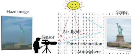
Suspended particles in atmosphere such as fog, murk, the mist, dust causes poor visibility image and distorts the colors of the scene. Haze image regards as a major challenge problem in many applications in the fields of image processing and computer vision. Hazy images can be modelled as a combination of scene radiance, Air light and transmission [1]. The study of haze is closely related to the works on scattering of light in the atmosphere. In imaging system, the main factors cause the image degradation can be due to atmospheric absorption, reflecting and scattering. In scattering some of incident energy redistributes due to exist of suspended particles into a total solid angle, as in figure 1 [2].

Figure 1: Effects Of Atmospheric Scattering

The main problem or challenge in de-hazing process is due to different density of haze from one region to other in the haze image, also the weather condition at the time of image capturing, The hazing images lose the color fidelity and contrast. Also the position of camera and how far from the sense may be cause for image degradation [3].

The task of image restoration is to estimate the latent high quality images given the low-quality observations.

Image de-hazing is one of the basic issues and more important research areas in the field of image processing and computer vision, the final goal of image de-hazing is to reconstruct visually pleasing images suitable for human visual perception, and to enhance the interpretability of images for computer vision and preprocessing tasks [4].

3636 statistical assumptions or priors. Among them, the method based on the dark channel prior (DCP) [5] achieves the state-of-the-art performance. Despite good performance, this method has some drawbacks. It estimates patch-wise transmission that does not preserve depth edges, and

thus de-hazing results in haloes around the object boundaries. To reduce the haloes, a transmission refinement step is necessary, which is either time consuming or less accurate [5]. In addition, for large bright surfaces, the DCP fails (treats the absence of dark pixels as the presence of haze) and overestimates the haze from its actual value, which causes over-de-hazing [6].

Since the dark channel prior is a kind of statistic, it may not work for some particular images. When the scene objects are inherently similar to the atmospheric light and no shadow is cast on them, the dark channel prior is invalid.

Our method will improve the way of estimation dark channel in addition to improve the estimation of the transmission factor to overcome these problem, and problem of objects which is like the sky or air light, such as the white marble. Also the paper works to reduce the haloes.

2. RELATED WORK

We will show some of the methods which have a significant role in explaining the problem and develop solutions for it.

Zhang introduced a developed atmospheric scattering model by dividing the hazy image according to the haze density, and defines a weight function to locate a candidate scene and improve the atmosphere light. Next combines with suggestion model named the average saturation prior (ASP), which depends on the average saturation probability distribution of hazy images with atmosphere light to guesses the scene atmospheric scattering coefficient and gets the scene albedo [7].

Cia, Bolun used Convolutional Neural Networks (CNN) relying on feature extraction to estimate a medium transmission map and offering a nonlinear function called Bilateral Rectified Linear Unit (BReLU) to enhance the quality of a de-haze image. Then making connections between the proposed DehazeNet and existing model [8].

Chen, Xumeng suggested a method depending on estimating illumination/reflection imaging model for hazing image. The first step in the suggested method is estimation of atmospheric veil based on the minimum intensity of RGB of each channel and enhances it by the guided filter. In the second, he computes the residual image by subtracting atmospheric veil from haze image. Finally he determine the maximum intensity in the residual which enhanced it by the guided filter to be as illuminating veil, Then divides the residual image by the illuminating veil to get an image free from haze [9].

3. HAZE MODELING

The observed brightness of a capture image in the presence of haze can be modeled based on the atmospheric optics [10] via

Ip= tp∙ Jp+ (1 − tp) ∙ A

where Jpand Ipdenote the original color and the

observed color at pixel position p, respectively,

and A is the airlight that represents the ambient light in the atmosphere. Also, tp ∈ [0, 1] is the

transmission of the light reflected by the object. Since the light traveling a longer distance is more attenuated, we have

tp= e−βdp

where βis the attenuation coefficient determined

by the weather condition and dp is the scene

depth from the camera. Thus, the reflected object

color Jpis attenuated by tp, whereas the air light

A is weighted by (1−tp) and plays a more

important role if the object is farther from the camera.

4. METHODOLOGY

The proposed algorithm suggested new method for image de-hazing based on the following steps:

1. Image filtering.

2. Determine the dark channel prior.

3. Estimating the Atmospheric Light.

4. Update the Atmospheric light value.

5. Estimating the transmission value.

6. Recover the de-hazed image.

7. Improve local contrast.

3637 Figure 2: Haze Image.

1. Image filtering

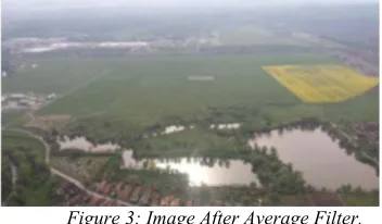
Filtering is a technique for modifying or enhancing an image. Image processing operations implemented with filtering include smoothing, sharpening, and edge enhancement. Average filter is suggested to replace each pixel by the average of pixels in a square window surrounding this pixel, in this paper we use small widow because the large window can remove noise more effectively, but also blur the details and edge, we need a trade-off between noise removal and detail preserving. For that we suggest 5x5 window using in (average filter) which give best results, image after filtering show in figure 3.

Figure 3: Image After Average Filter.

2. Determine the dark channel prior.

According to the literature report [8], based on the observation on haze-free outdoor images, in most of the non-sky patches, at least one color channel has very low intensity at some pixels, which is called the dark channel prior (DCP). In another word, the minimum intensity in such a patch should have a very low value, in this paper we use average instead of minimum to find the DCP. Dark channel determined by using the following formula

K x min

∈ , , average_∈ K i

Where K is a dark channel , Kc _{is an intensity of}

color channels R,G and B in image result from step 1, x is a center of a local patch Ω(x), the size of the local patch is 5*5.

From the dark channel process we get (2D) matrix with the same size of origin image as in figure 4.

Figure 4: The Dark Channel Image.

For the next step we need to select the top (1%) of pixels from dark channel matrix. This can be implemented by sort the value of dark channel in descending order, then we select the top 1% of the matrix values. With each value of the sorted top (1% pixels) we store the index (location in matrix).

3. Estimating the Atmospheric Light The image will be divided to many non-overlap blocks, each block with size (30x30). For each block determine the standard deviation:

s xi x

Where (s) is the standard deviation, (n) is the total numbers of pixels in block, (xi) is the

intensity of pixels and x is the mean of pixels

in block.

The standard deviation gives the amount of smoothness, thus gives the amount of variation in intensity of pixels. We can take the value of Air-Light from the sky region which has very low variation in intensity of pixels, that prevents us from taking the value of Air-Light from a white object founded in image.

At this case we compare the result of standard deviation with the top value of dark channel, then we select the value from the dark channel which correspond to the low standard deviation, which regards as the initial value of air light.

4. Update the Atmospheric light value

The next step is to enhance the value of Air light, this can be accomplished by the following way

1) Determine the standard deviation (Std_haze)

for the haze image ( RGB image).

2) Convert the haze image to HSV color space.

3) Determine the standard deviation for the (V)

3638

4) Find the global standard deviation which

equal:

St=Std_haze*Std_HSV.

5) Determine the average value of initial air

light components (R, G, B) (Av_of_Air).

6) Find the maximum value of dark channel

histogram (most frequency value in dark channel).

7) Find the max value of top lightest values

(1% pixels) histogram (most frequency value in top value of dark channel).

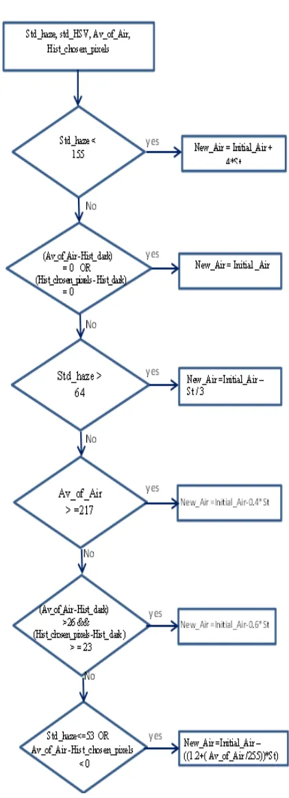
8) According to the previous values we modify

the initial Air light value according to the rules show in flow chart figure 5: (Note: these rules suggested according to experiments).

3639 5. Estimating the transmission value

After we find the final value of Air light, we

have to find the transmission value.

Transmission value can be determined by the following formula:

K x 1 w ∗ min

∈ , , average_∈

K i

The value of w is application-based. We fix it to

0.85 for all results reported in this paper, the result of this step show in figure 6.

Figure 6: The Transmission Map.

6. Recover the de-hazed image

Now, the important step is recovering the haze free image, the de-hazed images are recovered using the dichromatic model as follows [9].

k x H x A

max t x , to A

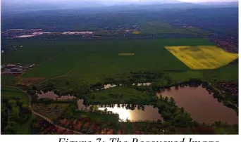
Where t0 is the lower bound for transmission map, t0=0.001 , we use t0 to prevent a very dense haze regions. Where the direct attenuation closes to zero when (t(x)) is very low, recover image show in figure 7.

Figure 7: The Recovered Image.

7. Improve local contrast

Improve local contrast is essential step in de-hazing process. Based on observation we conclude that we need the local contrast whenever dense haze was exists in image. For that, first we sharpen the RGB image. While in the second step we convert the image to (HSV color space), then we enhance the local contrast on the (V channel) by using the (Log filter), then

we reconstruct the RGB image, which represent the final result as show in figure 8.

Figure 8: Recovered Image After Enhance The Contrast (Final Result).

5.THE RESULTS

Before we show the results of test the proposed method, we must talk about the Qualitative Evaluation or metrics Evaluation. It is problematic to find universal measure to qualify of enhanced images and very hard to find metrics evaluation to measure the amount of de-hazing.

1. Measuring Image Quality

Generally, the image quality assessment (IQA) is divided into two classes; no reference and full reference.

A. No reference or blind quality:

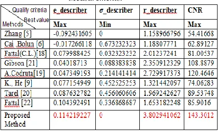
We will use the qualities suggested by Hautire [11] ( e , σ ,r) also we will use the Contrast to Noise Ratio (CNR).

a) e- Descriptor counts the numbers of visible edges in the de-haze image comparing with the haze image. Higher values means more visible edges in the de-haze image.

b) r_ Describer determine the ratios of the visible edges, that is shows the quality of the contrast restoration. Higher value means better contrast.

c) σ_ Descriptor count the number of pixels that are completely black or white after applying the de-haze method.

3640 Where (Ia) is the signal intensity of region a , (Ib) is the signal intensity of region (b and N) is the background noise.

B. Full reference:

In this section we will use the following measurements:

a. Root mean square error (RMSE) [13]:

1 ∗

√

b. Peak Signal to Noise Ratio (PSNR) [14] :

20 ∗ 10 2

√

c. Structural Similarity Index for

measuring image quality (SSIM) [15]:

SSIM

d. The universal image quality index

(UIQ ) [16]: The range of UIQ is [−1, 1], and the best value is one.

UIQ 4 Mx My Cxy

Mx My σx σy

Where (Mx) is the mean values of original image and (My) the mean values of distorted

image. Cxy is the covariance of both images.

(σx) the standard deviation of original and (σy) the standard deviation of distorted images. (c1, c2) are constants.

2. Test the Proposed Method

The proposed method tested by using more than 3000 haze image; 1200 images are chosen randomly from Internet, 420 images from FRIDA database (Foggy Road Image Database)

[17], and 1472 images from D-HAZY A

DATASET [18]. In this section we just display sample of images, and measuring the quality for another sample of images.

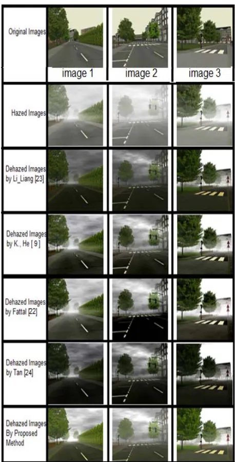
1. At first we compared the proposed method

visually with other methods and the results show in figure 9.

Figure 9: Visual Test For De-Hazing Images And Compared With Many Methods. (1) Haze Image. (2) Zang [7]. (3) Cai, Bolun [8]. (4) Fattal. [19]. (5) A.

Codruta [20]. (6) K., He [9]. (7) Tarel [21]. (8) Gibson [22]. (9) Fatal [23]. (10) Proposed Method.

In This Test It Is Clear The Image Result From Proposed Method Have More Quality From The Other

Images It Is Visually Pleasing Images Suitable For Human Visual Perception.

2. Using the quality measuring to test the

proposed method and compared the results with other methods as in table 1.

Table 1: Comparing The Proposed Method With Other De-Hazing Method By Using The Quality

Measurements.

3641 resolution and more contrast to noise ratio which mean less noise.

3. The third test we select some images

and add haze to them, then de-haze the images by proposed method and other methods, the results show the quality in tables 2, 3, and 4, and visually in figure 10.

Table 2: Performance Measure For Dehazed_Image 1.

Table 3: Performance Measure For Dehazed_Image 2.

Table 4: Performance Measure For Dehazed_Image 3.

This test used same amount of haze and de-haze the image by many methods. Table 2 show that the proposed method have more visible edges, best resolution and contrast, better quality when measuring PSNR (the quality is close to other methods), an same thing for other measures. SSIM and UQI can describe the information fidelity between the original image and the recovered image. Increase these values indicate more similarity between origin image and recovered image.

Results show that the algorithm is valid, fast, and suitable for the rapid de-hazing of numerous images.

Figure 10: Visual Test The Quality Of De-Hazing By Many Methods, When Add Haze To Origin Image.

It is clear that the proposed method better than other methods.

4. We compare the execution time for proposed

3642 Table 5: Comparing The Execution Time Among

Many Methods (Time In Sec), For Different Image Size [7].

From table 5 we conclude that the execution time for proposed method was reasonable and less than the execution time for other methods.

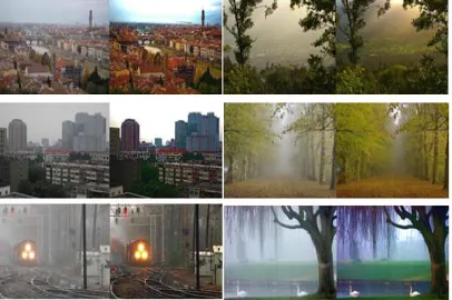
5. Figure 11 show sample of haze images

with corresponding of de-hazed images by using proposed method.

Figure 11: Some Of Well-Known Images Dehazed By Proposed Method.

Recovering the image as origin image may be regards as a very difficult challenge faces researchers due to many reasons. All algorithms now try to improve the image through de-hazing and recover more image contents and details. The suggested method improve the current algorithms and gives better results than other algorithms. From the quantitative results, the suggested method has a remarkable improvement on the quality of the recovered image. One advantage of this method is no haloes shows with de-hazed image.

6. CONCLUSIONS

In this paper we suggest new method for de-hazing images. The contribution of this paper is (1) estimate the dark channel prior based on average. (2) Estimate the value of Air light based on standard deviation (which is a result of standard deviation of RGB haze image and HSV color space haze image), we suggested many rules based on experiments. (3) We suggested to enhance the contrast by local contrast for (V) channel in the HSV color space. Results was very promised visually and by using some quality metrics. The proposed algorithm compared with other methods and it was more efficient in many situations. One of important enhancement in this paper is the removing of haloes. We think that the Air light need to enhance to recover some of de-haze problems, for that we suggest for future works to estimate the Air light by two or more methods and use the best one.

REFERENCES:

[1] Renjie He, Zhiyong Wang, Yangyu Fan and David Dagan Feng, “Combined constraint

for single image Dehazing”,

ELECTRONICS LETTERS, Volume 51, Issue 22, October 2015 ,pp 1776–1778.

[2] Lin-Yuan He, Ji-Zhong Zhao, Nan-Ning

Zheng, and Du-Yan Bi, “Hardy Variation Framework for Restoration of Weather Degraded Images”, Mathematical Problems in Engineering, Volume 2015, 2015 , pp 1-11.

[3] Dan Wang, Jubo Zhu, “Fast smoothing technique with edge preservation for single image dehazing”, IET Computer Vision, Volume 9, Issue 6, 2015 ,pp 950–959. [4] Bingquan Huo and Fengling Yin, “Image

Dehazing with Dark Channel Prior and Novel Estimation Model”, International Journal of Multimedia and Ubiquitous Engineering Volume 10, Issue 3, 2015 ,pp 13–22.

[5] He, K., Sun, J., Tang, X.: ‘Guided image filtering’. ECCV, 2010, pp. 1–14

3643 [7] Gu Z, Ju M, Zhang D. A Single Image

Dehazing Method Using Average Saturation Prior. Hindawi , Mathematical Problems in Engineering , 2017, pp 1–17.

[8] Cai B, Xu X, Jia K, Qing C, Tao D. DehazeNet: An end-to-end system for single image haze removal. IEEE Trans Image Process, Volume. 25, Issue 11, 2016, PP 5187-5198.

[9] Chen X. A Fast Algorithm for Single Image Dehazing Based on Estimating Illumination Veil. MEIC , 2015, pp 987-991.

[8] Bingquan Huo and Fengling Yin, “Image Dehazing with Dark Channel Prior and Novel Estimation Model”. International Journal of Multimedia and Ubiquitous Engineering , Volume 10 . Issue 3 , 2015, pp 13-22.

[9] He, K., Sun, J., and Tang, X.: ‘Single image haze removal using dark channel prior’, IEEE transactions on pattern analysis and machine intelligence, Volume 33 . Issue 12 , 2011, pp . 2341–2353.

[10] Jin-Hwan Kim, Jae-Young Sim, Chang-Su Kim, “Single image dehazing based on contrast enhancement”, Acoustics, Speech and Signal Processing (ICASSP), 2011 IEEE International Conference on, DOI:10.1109/ICASSP.2011.5946643. [11] Hautire, N. and Tarel, J.-P. and Aubert, D.

and Dumont E. “Blind Contrast

Enhancement Assessment By Gradient Ratioing At Visible Edges”. Image Analysis \& Stereology, Volume 27 , Issue 2, 2011, pp . 87–95.

[12] Levin A, Lischinski D, Weiss Y. “A closed-form solution to natural image

matting”. IEEE Trans Pattern . Volume 30 ,

Issue 2 , 2008, pp . 228–242

[13] Singh Y, Goyal ER. “Haze Removal in Color Images Using Hybrid Dark Channel Prior and Bilateral Filter”. International Journal on Recent and Innovation trends in Comp. and Comm, Volume 2 , Issue 12 , 2014, pp . 4165–4171.

[14] He K, Sun J, Tang X. “Guided Image Filtering (ECCV)”. European Confenrence on Computer Vision Volume 35 , Issue 7 , 2010, pp . 1–14

[15] Zhen C, Jihong S, Roth P. “Single image defogging algorithm based on dark channel priority”. Journal of Multimedia, Volume 8,

Issue 4, 2013, PP 432-438.

[16] Scholar MT. Remote Sensing Image Dehazing using Guided Filter. IJRSCSE, Volume 1, Issue 3, July 2014, PP 44-49. [17] Tarel JP, Hautière N, Cord A, Gruyer D,

Halmaoui H. “Improved visibility of road scene images under heterogeneous fog”. Intelligent Vehicles Symposium (IV) IEEE, 2010, pp 478–485.

[18] Ancuti C, Ancuti CO, De Vleeschouwer C.

D-HAZY: A dataset to evaluate

quantitatively dehazing algorithms. IEEE

International Conference on Image

Processing (ICIP) , 2016,pp 2226-2230. [19] Raanan Fattal, “ Dehazing Using

Color-Lines”, ACM Transactions on Graphics (TOG), vol. 34, issue 1, 2014, DOI: 10.1145/2651362.

[20] Codruta O. Ancuti, Cosmin Ancuti,

Chris Hermans, Philippe Bekaert, “A Fast Semi-inverse Approach to Detect and Remove the Haze from a Single Image”, Asian Conference on Computer Vision: Computer Vision – ACCV 2010 pp 501-514, DOI: 10.1007/978-3-642-19309-5_39. [21] Jean-Philippe Tarel, Nicolas Hautière, “Fast

visibility restoration from a single color or

gray level image”, Computer Vision, 2009

IEEE 12th International Conference on,

DOI:10.1109/ICCV.2009.5459251.

[22] Kristofor B. Gibson, Truong Q. Nguyen, “Fast single image fog removal using the adaptive Wiener filter”, Image Processing (ICIP), 2013 20th IEEE International

Conference on, DOI:

10.1109/ICIP.2013.6738147.