Quantifying uncertainty on sediment loads using bootstrap confidence intervals

www.hydrol-earth-syst-sci.net/21/571/2017/ doi:10.5194/hess-21-571-2017

© Author(s) 2017. CC Attribution 3.0 License.

Quantifying uncertainty on sediment loads using bootstrap

confidence intervals

Johanna I. F. Slaets1, Hans-Peter Piepho2, Petra Schmitter3, Thomas Hilger1, and Georg Cadisch1 1_{Institute of Plant Production and Agroecology in the Tropics and Subtropics, University of Hohenheim,} Garbenstrasse 13, 70599 Stuttgart, Germany

2_{Biostatistics Unit, Institute of Crop Science, University of Hohenheim, Fruwirthstrasse 23,} 70599 Stuttgart, Germany

3_{The International Water Management Institute, Nile Basin and East Africa Office,} Addis Ababa, Ethiopia

Correspondence to:Johanna I. F. Slaets ([email protected])

Received: 27 May 2016 – Published in Hydrol. Earth Syst. Sci. Discuss.: 21 June 2016 Revised: 6 December 2016 – Accepted: 23 December 2016 – Published: 27 January 2017

Abstract. Load estimates are more informative than con-stituent concentrations alone, as they allow quantification of on- and off-site impacts of environmental processes concern-ing pollutants, nutrients and sediment, such as soil fertility loss, reservoir sedimentation and irrigation channel siltation. While statistical models used to predict constituent concen-trations have been developed considerably over the last few years, measures of uncertainty on constituent loads are rarely reported. Loads are the product of two predictions, con-stituent concentration and discharge, integrated over a time period, which does not make it straightforward to produce a standard error or a confidence interval. In this paper, a lin-ear mixed model is used to estimate sediment concentrations. A bootstrap method is then developed that accounts for the uncertainty in the concentration and discharge predictions, allowing temporal correlation in the constituent data, and can be used when data transformations are required. The method was tested for a small watershed in Northwest Vietnam for the period 2010–2011. The results showed that confidence intervals were asymmetric, with the highest uncertainty in the upper limit, and that a load of 6262 Mg year−1had a 95 % confidence interval of (4331, 12 267) in 2010 and a load of 5543 Mg an interval of (3593, 8975) in 2011. Additionally, the approach demonstrated that direct estimates from the data were biased downwards compared to bootstrap median esti-mates. These results imply that constituent loads predicted from regression-type water quality models could frequently

be underestimating sediment yields and their environmental impact.

1 Introduction

The environmental impact of processes such as erosion, sed-imentation, eutrophication or degradation of aquatic ecosys-tems can only be quantified through reliable estimates of sed-iment, nutrient or pollutant loads (Walling and Webb, 1996). Monitoring constituent concentrations alone does not suffice as these provide information on in-stream quality but offer no means to evaluate outcomes such as reservoir siltation, ero-sion, soil fertility loss and pollution at the watershed scale – both on- and off-site. Despite abundant literature developing appropriate procedures for load estimates, most studies do not report a measure of uncertainty on the load (Kulasova et al., 2012).

uncertainty in the sediment concentration equation (the so-called sediment rating curve), and the uncertainty in the dis-charge, as discharge is usually not measured directly, but rather is predicted from a stage–discharge rating curve, with water level as the predictor variable. Any measure of uncer-tainty on the constituent load must take into account the un-certainty in both the constituent concentration and the dis-charge.

Uncertainty of the sediment concentration prediction has been extensively discussed and, depending on the catchment characteristics, generally good concentration predictions are obtained with errors smaller than 15 % (Horowitz, 2008). In some studies, however, the uncertainty is stated to be con-siderable. Smith and Croke (2005) for example reported that discharge only explained a quarter of the variability in the concentration data. Walling and Webb (1988) suggested that seasonal differences of the relationship between discharge (Q) and constituent concentration, non-simultaneity of Q

and concentration peaks during storms, hysteresis and ex-haustion effects are the most important causes of inaccuracy in concentration predictions. Few studies to date have taken this error on the discharge rating curve into account explicitly when calculating uncertainty on load estimates (Vigiak and Bende-Michl, 2013; Rustomji and Wilkinson, 2008). Uncer-tainties of discharge, however, depend on several factors: the method chosen to estimate the discharge, site conditions and the time interval over which water levels are measured (Harmel et al., 2009; Hamilton and Moore, 2012; McMillan et al., 2012; Tomkins, 2014). In general, discharge is esti-mated more accurately than constituent concentration. Dis-charge, however, enters the load equation twice – once as predictor variable for the concentration, and once multiplied with the concentration to get the instantaneous load. There-fore, it deserves further investigation whether or not the error on the discharge estimate can safely be ignored, and in which circumstances. Finally, as discharge is frequently used as a predictor for constituent concentration, the two variables are correlated and their errors cannot be assumed to be indepen-dent. As a result, there is no textbook formula to estimate the variance of a constituent load.

Therefore, authors that do report a measure of uncertainty often select a method that is specifically geared towards the application of load estimation at hand and not necessarily applicable to other sites, making it hard to compare results throughout the literature. Harmel et al. (2009), for exam-ple, developed a software tool to assess the errors introduced from estimating discharge, sample collection, preservation and storage, and lab analysis. In this tool, each of these sources is considered to be the result of random variability following a normal distribution. The sources of error are as-sumed to be independent of each other, and it is asas-sumed that the errors follow an additive law, but these assumptions will not apply in all situations.

Moatar and Meybeck (2005) assessed uncertainty on nu-trient loads by comparing loads based on a random

subsam-ple of measurement times, with a high-resolution load that is considered the “true” load. This approach is suitable for testing different methods and different temporal measure-ment resolutions of load estimation, but it does not assess the uncertainty of the “true” load, as it is assumed that, with sufficiently high sampling frequency (in their case, daily), the measured load is equivalent to the actual load. More re-cently, two new candidate approaches have emerged to calcu-late confidence intervals on loads that have the potential to be generally applicable, regardless of the method used to calcu-late the load and the distributional assumptions made: boot-strap methods (Mailhot et al., 2008; Rustomji and Wilkinson, 2008; Vigiak and Bende-Michl, 2013) and Bayesian methods that result in credibility intervals (Pagendam et al., 2014; Vi-giak and Bende-Michl, 2013).

The bootstrap is a Monte Carlo-type method, where a large number (B) of datasets are simulated – either by sampling with replacement from the original data in the case of the non-parametric bootstrap or by sampling from a fitted dis-tribution in the case of the parametric bootstrap (Efron and Tibshirani, 1993). Bootstrap methods, however, were origi-nally developed for independent, identically distributed ran-dom variables. In the context of sediment monitoring the as-sumption is that the observations used to build the regression model are independent in time. This can be realistic in fixed-interval sampling schemes where the sampling time inter-val is large, or in the case of discharge where measurements to build the stage–discharge relationship are typically taken far apart in time. For sediment concentration, however, flow-proportional sampling is often performed to obtain samples at the highest concentrations. Those observations are usually taken closely together during storms and thus most likely are not independent in time (Slaets et al., 2014). Linear mixed models that model the serial correlation provide an alterna-tive to least squares regression to establish a sediment rating curve for this type of data. Lessels and Bishop (2013) sim-ilarly found that the inclusion of a temporal autocorrelation component improved the accuracy and decreased the bias in predictions of total phosphorus and nitrogen river loads. If there is serial correlation in the sediment data, it is neces-sary to use an adjusted version of the bootstrap that retains the serial correlation in the data intact (Lahiri, 2003). Such methods have already been explored in hydrology in relation to the discharge rating curve: Ebtehaj et al. (2010) and Selle and Hannah (2010) use block bootstrap methods to assess uncertainty in and improve robustness of model parameter estimates for discharge prediction.

safely be neglected in certain circumstances, and how they affect the resulting confidence intervals. The corresponding code in SAS was created and is available online to accommo-date these different scenarios (https://www.uni-hohenheim. de/bioinformatik/beratung/index.htm).

Our specific aims were: (i) to establish a generally appli-cable method to calculate confidence intervals on constituent loads, using bootstrap methods, (ii) to account for serial cor-relation in the data, (iii) to assess whether or not the effect of the uncertainty on discharge is negligible, (iv) to evaluate how data transformations affect the calculations, and (v) to determine the number of bootstrap replicates required to ob-tain reliable confidence intervals. Combining these aspects, the proposed method provides a means to assess uncertainty on any type of constituent load which was calculated from continuous constituent concentration and discharge predic-tions estimated with regression-type methods. The approach thus allows load estimates to be reported with an uncertainty assessment, rather than as a point estimate alone, making them informative to end users and decision makers.

2 Material and methods

2.1 Discharge and sediment concentration

Discharge and suspended sediment concentrations were con-tinuously monitored for a period of 2 years (1 January 2010– 31 December 2011) in a small agricultural catchment in mountainous Northwest Vietnam. The catchment is located in the Chieng Khoi commune (21◦₇0₆₀00_{N, 105}◦₄₀0₀00_E, 350 m a.s.l), Yen Chau district, in the tropical monsoon belt where the rainy season begins in April and ends in Octo-ber. Average annual precipitation is around 1200 mm; aver-age annual temperature is 21◦C. The occurrence of typhoons is not uncommon especially at the end of the rainy season, and daily rainfall amounts can rise to 200 mm. The largest storm during the 2 years of this study was on 12 July 2011 and consisted of 73 mm of rainfall in 3 h. The dominant soils are Alisols and Luvisols (Clemens et al., 2010). The land-scape has an altitudinal range between 320 and 1600 m a.s.l. with slopes ranging from 0.05 to 65 %. The measurement lo-cation is in a river at the outlet of a small watershed with a contributing area of 2 km2, of which 0.6 km2consist of paddy fields. A 26.3 ha surface reservoir with a buffering capac-ity of 106m3 provides irrigation water for rice production via concrete irrigation channels, and the paddies drain into the monitored river. As the reservoir fills up with the pro-gression of the rainy season, excess water is removed via a spillover which drains into the river, typically from July till October. During this period, discharge in the river is an or-der of magnitude larger than during times when the spillover is not active: mean daily discharge in the dry season equaled 0.08 m3s−1(with a standard deviation of 0.13 m3s−1), while

mean daily discharge with the spillover active amounted to 1.22 m3s−1_{(with a standard deviation of 0.66 m}3_s−1_).

For the discharge monitoring, water levels were mea-sured every 2 min for the river station using pressure sensors (EcoTech, Germany). The stage–discharge relationship was established with the velocity-area method (Herschy, 1995), where the velocity is measured with a propeller-type current meter (OTT, Germany) at one or more points in each vertical, depending on the water depth. The discharge is subsequently derived from the sum of the product of mean velocity, depth and width between verticals. Discharge measurements were never taken on the same day, and the closest time interval between two measurements was 1 week. The estimated dis-chargeQˆ in m3s−1at timeiwas then predicted from logQiˆ =logαˆ+ ˆγlog(hi−β) , (1) wherehi is the water level (in m) at timei,αˆ andγˆ the esti-mated rating curve constants andβ the measured sensor off-set, withαˆ andγˆestimated using the method of least squares on the log-transformed scale. This transformation was done to stabilize the variance.

As the irrigation management disturbed the natural rela-tionship betweenQand SSC, a turbidity-based method was used to monitor SSC. Turbidity was measured every 2 min with NEP395 sensors (McVan, Australia); 228 water sam-ples were collected using a storm-based approach, by taking around 20 grab samples per sampled rainfall event in order to accomplish the best possible coverage of all concentra-tion ranges; 188 storm-flow samples were collected during 24 rainfall events over the 2-year duration of the study. Ad-ditionally, every 2 weeks a base-flow sample was taken. The sediment concentration was determined gravimetrically on a sample of 500 mL by letting it settle overnight in refriger-ated conditions, prior to siphoning off the supernatant and drying the remaining sediment at 35◦C, as is recommended for samples with very high sediment concentrations (ASTM, 2013).

Rainfall was quantified with a tipping-bucket rain gauge on a weather station (Campbell Scientific, USA). Events were defined based on rainfall data (no pause in precipita-tion for longer than 30 min) and lag times were added based on cross-correlation analysis as described in Schmitter et al. (2012). A total of 420 rainfall events took place and were monitored during the 2-year study period.

based on the Akaike information criterion (AIC). The model uses turbidity and discharge as quantitative predictor vari-ables, and accounts for serial correlation. As surface reser-voir irrigation management was present in the watershed, classic variables related to catchment characteristics such as hysteresis patterns and exhaustion effects were not suitable predictors of sediment concentration. The predictor variables turbidity and discharge were also log transformed. All sam-ples from the 2-year study period were used to build the con-centration prediction model, and load estimates from both years are thus predicted from the same model with the same parameter estimates. All statistical analyses were performed using the MIXED procedure of SAS 9.4, which can fit linear models with more than one random effect. The covariance structure used to model serial correlation in the present study was a first-order autoregressive (AR(1)) model, which was selected based on the AIC. Assumptions of normality and homogeneity of variance were checked visually using diag-nostic plots.

Conceptually, the concentration prediction error can also be separated into an underlying latent autoregressive process generating the true concentrations, and an independently dis-tributed measurement error corresponding to white noise in time series data. The white noise is equal to the error that would remain if two measurements were conducted at al-most coinciding time points. This variability is typically at-tributable to measurement error and in spatial statistics, this is what is known as a nugget effect. In the MIXED proce-dure, this effect was fitted by using the local option in the repeated statement.

Validation was performed using 5-fold cross validation, in which the dataset is split randomly into five parts, and each part is used four times to calibrate the model, and one time for validation, so that each observation in the dataset is used for validation once. Pearson’s correlation coefficient (r) was calculated between the observed and predicted values resulting from the validation. A SAS macro that performs

k-fold cross validation (k=5 in our case) for linear mixed models using the MIXED procedure is described in Slaets et al. (2014). Additionally, event-based 5-fold cross validation was performed, where all samples belonging to single events were resampled jointly, rather than individual observations. 2.2 Bootstrap resampling procedure

In the non-parametric bootstrap, a large number (B) of ran-dom samples, of the same size as the original dataset, is drawn by sampling observations with replacement from that original dataset. For each of the B bootstrap samples, the sample statistic of interest (in this case, the sediment load) is calculated and from the resulting empirical distribution, measures of uncertainty can be obtained. As this empirical distribution is only a good approximation of the true distri-bution when the bootstrap resampling mechanism is able to recreate the original sampling process (Efron and Tibshirani,

1993), we need to understand the sampling processes result-ing in the annual sediment load. Since neither discharge nor constituent concentration are measured continuously, annual loads are normally estimated by calculating the sum of in-stantaneous loads, measured at equally spaced discrete points in time. The load at a timeiis then generated from

ˆ

Li= ˆQi× ˆCi, (2)

where Lˆi is the estimated instantaneous load at time i in

g s−1,Qˆi is the estimated discharge at timeiin m3s−1and ˆ

Ciis the estimated concentration at timeiin g m−3. These

in-stantaneous loads are multiplied by a time factor accounting for the monitoring interval. In the present study, for exam-ple, the factor was 120 s, as measurements were done every 2 min. Monthly or annual loads in Mg can then be calcu-lated by simply summing up the instantaneous loads for the whole time interval and multiplying by a factor 10−6_to con-vert from mg to Mg:

ˆ L1 tot=

Xt i=1(

ˆ

Li×120×10−6). (3)

Looking at Eq. (2) for the load estimate at a time i, there are really two separate sampling processes from two distinct populations at work in the load estimation: firstly the sam-pling for the discharge rating curve (pairs ofQandhfrom the full time series ofQandhpairs), and secondly, the sam-ples used to build the sediment rating curve (observations of

Cand hydrological predictor variables from the full time se-ries ofC,Qand turbidity). In order to assess the uncertainty of the discharge equation, the bootstrap replicates can be cre-ated by simply sampling (Q,h) pairs at random with replace-ment from the original dataset. Simple random resampling assumes independence, which is dependent on the monitor-ing scheme: in the case of our dataset, discharge measure-ments were never taken on the same day, and the smallest interval between two measurements was 1 week. In order to test this assumption, an AR(1) variance–covariance structure was fitted to the discharge data. As the AIC showed an in-crease of two points compared to an independent structure, no serial correlation was present in the (Q,h) pairs. Using Eq. (1), bootstrap dischargesQˆ∗_i can be generated according to

logQˆ∗_i =logαˆ∗+ ˆγ∗log(hi−β), (4)

wherehi is the water level at timei,β is the measured sen-sor offset, andαˆ∗ andγˆ∗are the bootstrap estimates of the discharge rating curve parameters. TheseB predictions of

often collected in a storm-based approach, as was done in this study, where they were collected sometimes only min-utes apart during rainfall events. For these types of hydro-logical datasets where temporal autocorrelation is present, Ebtehaj et al. (2010) recommended the use of specialized sampling procedures that keep the serial correlation intact, such as the moving block bootstrap, the circular block boot-strap or the stationary block bootboot-strap, described in detail by Lahiri (2003) and applied to constituent concentrations by Hirsch et al. (2015).

Among these specialized methods, no preferred method has emerged from the literature. Furthermore, many of these methods require a vast set of decisions such as for exam-ple the block size for which no general recommendation ex-ists. As a consequence, results from different methods are not straightforward to compare. As the goal of the bootstrap is to mimic the original sampling process, however, there is an in-tuitive choice in the case of event-based sampling: the rainfall events form natural “blocks” or sampling units, which is why water quality models used to predict continuous time series and thus new events should be validated on an event basis, rather than on a sample basis (Lessels and Bishop, 2013). So rather than sampling with replacement from the individ-ual observations (water samples representing a single time point), all samples belonging to one event can be resampled with replacement, thus keeping all observations within one event together and maintaining the serial correlation intact.

On the other hand, base-flow samples are typically taken at fixed time intervals far apart in time (here every 2 weeks). They can therefore be considered to be independent and can be resampled by simple random sampling with replace-ment, thus bootstrapping individual water samples from sin-gle time points. In a previous model published in Slaets et al. (2014), we explored the use of several alternative variance–covariance structures to model the serial correla-tion. The selected spatial power model unfortunately caused non-convergence for a large number of the bootstrap repli-cates when using it for bootstrap load estimates, and there-fore the AR(1) structure was implemented as it did not have convergence issues. The difference in AIC between the AR(1) and spatial power models was four points. Therefore the spatial power model is most likely the best performing model, but there is still considerable support for the AR(1) model (Burnham and Anderson, 2002). The spatial power structure with time as the coordinate showed that the auto-correlation becomes nearly zero for samples taken more than 80 min apart – which coincides with the average duration of rainfall events. Therefore the base-flow samples were consid-ered to be independent. An increase in AIC of one point when fitting a first-order autoregressive covariance structure con-firmed the lack of serial correlation in the base-flow samples. By resampling events with replacement for the storm-flow samples and observations with replacement for the base-flow samples,B time series of predicted sediment concentration

ˆ

C_i∗are generated from

ˆ

C_i∗= ˆδ∗+(νˆ∗)TXi, (5)

withδˆ∗ andνˆ∗the bootstrap estimates of the intercept and the regression coefficients, respectively,(νˆ∗)T the transpose of vectorνˆ∗andXithe design vector of the fixed effects. This is a generalized equation applicable to any linear model, re-gardless of the number of predictor variables. If the sediment concentration was predicted using turbidity and discharge, for example, the bootstrap time series of predicted sediment concentration would be generated from

ˆ

C_i∗= ˆδ∗+ ˆη∗Qˆ∗_i + ˆκ∗Ti, (6)

whereηˆ∗ is the bootstrap parameter estimate of the regres-sion coefficient for_Qˆ∗

i, the bootstrap discharge at timei

gen-erated from Eq. (4), andκˆ∗the bootstrap parameter estimate of the regression coefficient for Ti, the turbidity at timei,

respectively.

This resampling process accounts for the uncertainty that arises from estimating the parameters of the sediment rating curve from a dataset with a limited number of observations. If there were an unlimited number of water samples avail-able, the uncertainty of these parameter estimates would de-crease to zero. But it is more realistic to assume that, even if there were a very large number of samples available, there would still remain scatter in the real constituent concentra-tions around the equation, as the equation simply does not fully explain all the variation in sediment concentration. Sed-iment loads vary not only with discharge, but also with up-stream sediment supply, which in turn depends additionally on geology, soil types, land cover and land use change or management, all influencing sediment quantity and quality (Walling, 1977). Therefore, there is a fundamental reason for the scatter in the data: sediment loads are inherently non-capacity loads. Even if there were an unlimited number of samples available, this would not result in a perfect equation to predict sediment concentration. Therefore this additional uncertainty needs to be taken into account. For the discharge rating curve, if the river bed is stable and the stream bank vegetation does not change, the stage–discharge equation has a high accuracy and it is reasonable to assume the only error in the equation is measurement error; therefore, this addi-tional uncertainty is not a concern.

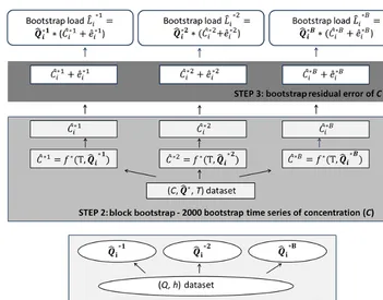
Figure 1.Flowchart showing the three-step bootstrap mechanism.

how large the observed dataset would be. However, by ran-domly resampling from the residuals, it is assumed that these residuals are independent.

When this assumption does not hold because samples are taken very closely together in time, as was the case for our dataset, the method can be modified so that the added errors reflect the temporal autocorrelation. To this end, the covari-ance parameter estimates from the original sample can be used as plug-in estimates. In the present dataset, an AR(1) structure was fitted to the data (Verbeke and Molenberghs, 2009), resulting in two covariance parameter estimates: one for the autocorrelation parameter (ρ)ˆ and one for the resid-ual error variance (σˆ_e2). The restricted maximum likelihood algorithm was used to simultaneously estimate the fixed ef-fects and the covariance structure (Patterson and Thompson, 1971). The use of the covariance parameter estimates ob-tained assuming a normal distribution of errors implies that the method is partly parametric. This is necessary in order to take the serial correlation in the data into account. The boot-strap error terme∗at timeiwas then generated according to the following equation:

ˆ

e∗_i = ˆρ∗eˆ∗_i−1+ q

(1− ρˆ∗2

)×f_i∗, (7)

whereρˆ∗is the bootstrap estimate of the autocorrelation pa-rameter, and the errorf_i∗was randomly drawn from a normal distribution with mean zero and a bootstrap variance(σˆ_e∗)2. The bootstrap prediction of a sediment concentration at time

i, including the error expected due to residual scatter in the data, is then given by

ˆ

C_i∗+ ˆe∗_i = ˆδ∗+(νˆ∗)TXi+ ˆρ∗eˆ∗i−1+ q

(1− ρˆ∗2

)×f_i∗. (8) In summary, the complete bootstrap process that accounts for uncertainty in the parameter estimates of both the discharge and sediment rating curves and uncertainty due to residual scatter in the sediment concentrations consists of three steps (Fig. 1):

1. resampling with replacement from the (Q,h) pairs B

times, in order to getBbootstrap stage–discharge equa-tions; applying these equations to the continuous water level data to obtainBbootstrap time series (Q∗)for dis-charge;

2. block-bootstrapping the (C, turbidity, Q∗, rainfall) dataset by drawing whole events and base-flow sam-ples with replacement, in each replicate plugging in the corresponding bootstrap Q∗ from Step 1, in order to getB bootstrap sediment rating curves; then applying these bootstrap sediment rating curves to the continuous turbidity,Q∗, and rainfall data to obtainB time series for the continuous suspended sediment concentration; and

In order to obtain a bootstrap estimate of the instantaneous loadLat timei, the equation is

ˆ

L_i∗= ˆQ∗_i ×(Cˆ_i∗+ ˆe∗_i). (9) The residual scatter on the discharge is not added, as the stage–discharge rating curve has a much higher accuracy on the one hand, and on the other hand, velocity measurements are typically taken quite far apart in time, which would not allow modeling of the serial correlation of the time series for discharge, but this would be needed because of the shortness of the time intervals considered here (2 min).

Finally, these bootstrap instantaneous load estimates can be summed up for the whole time interval, resulting in B

estimates of monthly or annual loads:

ˆ

L∗_{1 tot}=Xt i=1(

ˆ

L∗_i ×120×10−6). (10) 2.3 Data transformations

If the data are not normally distributed, it can be necessary to transform variables, as was done for this dataset with a Box– Cox transformation. In this case, the variables in question can simply be transformed before starting the bootstrap, and all the bootstrap estimates are obtained on the transformed scale. The back-transformation is then performed in Eq. (9) to obtain load estimates on the original scale. For example, in a typical case where both discharge and sediment concen-tration need to be log-transformed, the bootstrap predictions of discharge in Eq. (4) and of concentration in Eq. (8) will be on the log scale. These predictors then need to be back-transformed to the original scale using the inverse of the log-arithm.

This approach is applicable to any type of data transforma-tion, and thus offers a flexible framework that can accommo-date different methods of estimating the constituent concen-tration. However, if a modeled residual error term eˆ_i∗is not included, care must be taken with the back-transformation. With nonlinear data transformations (the log-transformation and the Box–Cox transformation being prime examples), predicted means cannot be naïvely back-transformed and in-terpreted as means on the original scale. Correction factors can be applied that compensate for the underestimation of SSC that arises from doing the predictions on the trans-formed scale. A commonly used non-parametric correction factor is Duan’s smearing estimator (Duan, 1983), where the sample average of the exponentiated residuals from the model is used as the correction factor. Duan’s smearing es-timator assumes independent and identically distributed er-rors, however, and is therefore also not a suitable alternative when serial correlation in the data is present. Alternatively, as pointed out by Rustomji and Wilkinson (2008), adding the modeled residual error removes the need to apply a cor-rection factor and is therefore the recommended approach. Regardless of the chosen correction factor, it is important that homoscedasticity after the transformation is confirmed

by visually inspecting the diagnostic plots, as was done in the case of this dataset. While discharge is also typically predicted on the log-transformed scale, in our dataset the variance was much smaller than that of the concentration data. With a small variance, the log-normal distribution is nearly normal and, therefore, the naïve back-transformation of log(Qˆi)should approximate the mean well.

2.4 Alternative option to simulate errors

If a data transformation is required and one does not want to explicitly simulate the residual scatter, then a correc-tion factor must be applied to the back-transformed concen-tration. This correction is needed because the naïve back-transformation (for example, taking the exponent of the pre-dictions if the prepre-dictions are on the log scale) does not yield a predicted mean, but rather a predicted median. While me-dians can be informative measures of a central tendency to skewed datasets, they are not appropriate when the objective is to calculate a constituent load: loads are sums over equally spaced time points, and in order to obtain an unbiased es-timate of this sum over time intervals, we need to sum up estimates of the expected values, rather than the medians, for each interval.

The required correction factor is specific to the type of data transformation. For a logarithmic transformation, the expected value can be obtained by adding on half of the residual error variance to the predicted concentration on the log scale before back-transforming. For other cases of the Box–Cox transformation, the correction depends on the se-lected transformation parameter. Solutions for specific exam-ples of the transformation parameter can be found in Free-man and Modarres (2006). As the selected transformation in this dataset was the logarithm, the correction of adding half the residual error variance before back-transforming was compared to the approach where the error is simulated, in or-der to see how this affects sediment load estimates and the resulting confidence intervals.

2.5 Bootstrap confidence intervals

A straightforward way to calculate a confidence interval (CI) on a parameter after bootstrapping is the bootstrap percentile method (Efron and Tibshirani, 1993). If a 95 % CI is re-quired, the confidence interval would simply be calculated by ordering the bootstrap load estimates from small to large and taking the 2.5th and 97.5th percentiles as the lower and upper limits.

large number of bootstrap replicates (upward of 500) are usually required to achieve acceptable accuracy (Efron and Tibshirani, 1993). How many exactly depends on the statis-tic in question, and should be empirically tested for each case: when the process is repeated, the resulting CI should not greatly differ, otherwise the number is too small. In the present dataset, a choice of 2000 bootstrap replicates yielded replicable results.

Improving upon the bootstrap percentile method, Efron and Tibshirani (1993) proposed bias-corrected and acceler-ated intervals, used by Vigiak and Bende-Michl (2013). Un-fortunately, this approach requires an even larger number of bootstrap replicates than the percentile method to suffi-ciently reduce the Monte Carlo sampling error. This is a dis-advantage when working with hydrological time series, as the datasets typically contain a large number of records al-ready. This method then quickly becomes time consuming, and therefore in this paper, preference was given to the more intuitive and less computationally intensive bootstrap per-centile method.

2.6 Identifying hydrological drivers of uncertainty The proposed three-step bootstrap process offers an opportu-nity to assess the importance of different aspects of the load calculation for the accuracy of the estimate. By leaving out step 1 (bootstrapping theQ−hpairs) and just usingQas pre-dicted by the discharge rating curve from all observed data points, confidence intervals can be obtained that only take into account the uncertainty on the sediment rating curve. If the resulting confidence intervals closely resemble the confi-dence intervals calculated with the full approach, this would mean that the uncertainty in the sediment concentration is what drives the uncertainty in the loads, thus supporting the finding that the error in the discharge is negligible compared with other sources of uncertainty (e.g., Némery et al., 2013, Vigiak and Bende-Michl, 2013).

As the accuracy of the stage–discharge relationship de-pends on the type of streambed, the method chosen and the number of measurements taken, this assumption might also hold true for some watersheds such as the one in this study, where the relationship had a highR2, but not for others. To determine at which point the uncertainty inQmust be taken into account for the load confidence interval, datasets of (Q,

h) pairs were simulated with decreasingR2(0.95, 0.90, 0.85 and 0.80), and were each used as an input dataset for boot-strapping the stage–discharge relationship (Step 1 in Fig. 1) in order to test the sensitivity of the confidence intervals to the accuracy of the discharge rating curve. The datasets with a fixed realizedR2 were simulated by a rescaling of errors which is described in Appendix A, and SAS code to perform the simulation can be found in the Supplement.

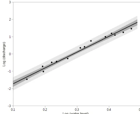
Figure 2. Discharge rating curve plotted on the log-transformed scale showing the 95 % confidence interval for the regression line (dark grey) and for new predictions (light grey). Stage–discharge rating curve: log(discharge)=(9.0819·log(water level))−2.6423 (n=15,R2=0.98).

3 Results

3.1 Rating curves and load estimates

The coefficient of determination of the stage–discharge rela-tionship was 0.98 (n=15, Fig. 2). Homoscedasticity was ob-served on the log-transformed scale (Fig. 3). For the sediment rating curve, Pearson’s r between observed and predicted values on the log-transformed scale wasr=0.75 after 5-fold cross validation (n=228, Fig. 4). Event-based cross valida-tion yielded very similar results, demonstrating the robust-ness of the model (r=0.77). The sediment rating curve tends to overpredict low concentrations and underpredict high con-centrations for new data, as is visible in Fig. 4. This tendency of regression towards the mean is typically seen when mod-els are fitted to very noisy data, and is also well documented in erosion studies (Nearing, 1998). Thus, in the case of our dataset, the discharge rating curve explained a higher pro-portion of the variance than the sediment rating curve, as is typical. Again, homoscedasticity was observed on the log-transformed scale (Fig. 5). The bootstrap parameter estimates forρ of the AR(1) process varied from 0.56 to 0.93 with a mean of 0.77, showing the block bootstrap kept the serial correlation intact as required.

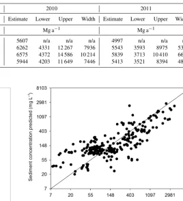
back-Table 1.Annual sediment load estimates (in Mg per year) for the 2 years of the study directly estimated without bootstrapping, and load estimates with 95 % confidence interval limits and interval widths (difference between the upper and lower limits) for the three different boot-strap methods: the full method shown in Fig. 1, the method without modeled error (i.e., leaving out Step 3 in Fig. 1) and the method without bootstrapping discharge (i.e., leaving out Step 1 in Fig. 1) (n/a: not applicable).

Error source 2010 2011

Method Autocorrelation Q-equation Estimate Lower Upper Width Estimate Lower Upper Width

Mg a−1 Mg a−1

Direct estimate 5607 n/a n/a n/a 4997 n/a n/a n/a

Full bootstrap method X X 6262 4331 12 267 7936 5543 3593 8975 5383 Bootstrap without modeled error X 6575 4372 14 586 10 214 5839 3713 10 410 6697 Bootstrap without discharge X 5944 4203 11 649 7446 5413 3521 8394 4876

Figure 3. Residual plot for the discharge rating curve, showing studentized residuals versus the predicted discharge (on the log-transformed scale).

transformation. Second, the median of the bootstrap esti-mates of the sediment load was taken, where, identically to the first case, the concentrations were corrected by adding half the residual error variance before back-transforming (Bootstrap without modeled error in Table 1). Third, the me-dian of the bootstrap estimates was taken for the bootstrap process that included a modeled, autoregressive error term (Full bootstrap method in Table 1).

For this last estimation method, the annual sediment load was estimated to be 6262 Mg in 2010 and 5543 Mg in 2011 (Table 1). When the median from the bootstrap sediment load estimates was taken without modeled error, but rather apply-ing the back-transformation correction, the load was approx-imately 5 % higher for both annual and monthly load esti-mates (Table 1 and Fig. 6). The annual loads thus amounted to 6575 Mg in 2010 and 5839 Mg in 2011. Finally, if sedi-ment loads were estimated not by bootstrapping, but directly from the data, then the results were around 10 % lower

com-Figure 4. Observed versus predicted values of the sediment rat-ing curve. Predictions are from the linear mixed model with tur-bidity and discharge as quantitative predictor variables, and after 5-fold cross validation (n=228,r2=0.56). Axes are on the log-transformed scale, while tick labels show values on the original scale.

pared to the first estimates, at 5607 and 4997 Mg, respec-tively, in 2010 and 2011.

In all three approaches the difference between the 2 years remained consistent and all estimates were within the bounds of the confidence intervals, both for those calculated by mod-eling error and those calculated by adding half the variance before back-transformation.

Figure 5. Residual plot of the sediment concentration prediction model; studentized residuals versus the predicted sediment concen-tration (on the log-transformed scale).

(Slaets et al., 2015). True upland area erosion rates were es-timated at 7.5 Mg ha−1a−1(Slaets et al., 2015).

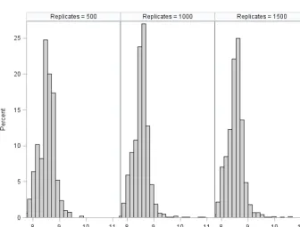
3.2 Width of confidence intervals for sediment loads Before looking at the bootstrap confidence intervals, the histograms of the bootstrap load estimates were evaluated (Fig. 7). The histogram of the 2000 bootstrap estimates looked reasonably smooth, so we concluded that sample size was adequate for the percentile bootstrap. When reducing the number of bootstrap replicates (Fig. 8), the change in smoothness, especially in the right tail, becomes visible. Tail smoothness of the empirical distribution is a requirement when using the percentile method to obtain confidence in-tervals (Efron and Tibshirani, 1993). At 500 bootstrap repli-cates, the center of the distribution displays a lack of smooth-ness as well, thus not only affecting the confidence interval estimates, but the load estimates as well. For both years and both for the full method and the method without modeled error, the histograms were found to be skewed to the right, even when the loads were log-transformed. This skewedness means that, in the case of our dataset, the assumption of nor-mality would not hold for estimated annual loads.

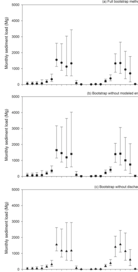
As a result of the distribution of the loads, the confidence intervals were always asymmetric, with the difference be-tween the upper limit and the estimate around 80 % larger than the difference between the estimate and the lower limit. The width of the intervals – the difference between the up-per and lower limits of the interval – varied between years and between methods, while remaining on the same order of magnitude (Table 1). In 2010, the interval was always wider, regardless of which method was chosen, for the annual as well as the monthly loads (Table 1 and Fig. 6). The year

Figure 6.Monthly sediment load estimates (in Mg per year) for the 2 years of the study with 95 % confidence interval limits for the three different bootstrap methods:(a)the full method shown in Fig. 1,(b)the method without modeled error (i.e., leaving out Step 3 in Fig. 1) and(c)the method without bootstrapping discharge (i.e., leaving out Step 1 in Fig. 1). In January 2011, discharge was zero; therefore, no sediment load was transported during this month.

Figure 7.Histograms of bootstrap load estimates on the original scale (left) and the log scale (right) for 2 study years and for two bootstrap methods: the full method with modeling of the autocorrelated error (“full method”, top), and without modeling of the error (“no md. err.”, bottom).

Figure 8.Effect of the number of bootstrap replicates (1500, 1000 and 500) on the smoothness of the resulting empirical distribution for the estimated annual sediment load in 2011.

The bootstrap method affected the width of the confidence interval as well. The monthly and annual intervals resulting from applying a back-transformation correction were

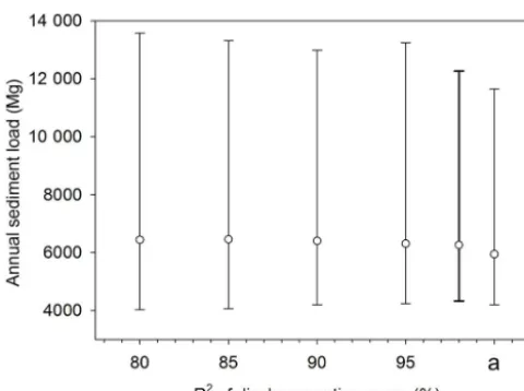
Figure 9.Change in the median and 95 % confidence intervals for the sediment load estimate of 2010 (in Mg) when decreasing the coefficient of determination of the discharge rating curve. The bold line indicates the CI width of the real (discharge, level) dataset. The letter “a” corresponds to not bootstrapping the (discharge, level) pairs.

to (4372, 14 586) in 2010 and from (3593, 8975) to (3713, 10 410) in 2011 – in both cases an increase in width of about 20 %. The change was due to an increase in the upper bound of the interval, while the lower limits remained very similar. These results show that performing the back-transformation correction is only a very rough method of adjusting the pre-dicted concentrations on the original scale, as this approach does not take the serial correlation in the data into account. For the monthly load estimates, the largest differences in confidence interval width between the full method and the back-transformation without simulated error were in July and August 2010, the months with the highest estimated loads (Fig. 6).

3.3 Hydrological drivers of uncertainty

When, rather than applying the full bootstrap method, we did not bootstrap the discharge rating curve (meaning, we left out Step 1 of the process in Fig. 1), the width of the confidence interval decreased, as one less source of error is taken into account. In 2010, this changed the CI from (4203, 11 649) without accounting for uncertainty in the discharge rating curve to (4331, 12 267) when accounting for this uncertainty on discharge; and from (3521, 8397) to (3593, 8975) in 2011 – including discharge therefore resulted in a respective in-crease in width of 6 and 9 %. Similarly, in the monthly load estimates, not bootstrapping the discharge resulted in confi-dence interval widths up to 37 % smaller than those calcu-lated with the full method (Fig. 6). Months with low flow showed equally compressed confidence intervals as months with high discharge, during which the reservoir spillover was feeding the river (July till October).

The accuracy in the (Q, h) relationship in this particu-lar dataset was very high, with an R2 of 0.98. As not all monitoring programs can establish accurate discharge rat-ing curves, the (Q, h) dataset was replaced with a simulated dataset with an increasingly lower coefficient of determina-tion to test how this further affects the uncertainty in the load estimate (Fig. 9). While the width of the confidence interval keeps increasing with decreasingR2, including the discharge also affects the confidence interval for a high R2. In fact, changing from not bootstrapping the discharge (R2=100 % in Fig. 9) to bootstrapping the real discharge dataset, which has anR2of 0.98, resulted in a 7 % increase in width. On the other hand, the confidence intervals show little differences at anR2 of 0.95, where the width was 9003 Mg, and at 0.90, when it reached up to 8795 Mg, equivalent to an 11 % in-crease in width. At a coefficient of determination of 0.85, the CI was 17 % wider than the original CI, whereas at 0.80 the width increase reached 20 %. As can be seen from Fig. 9, the change in width was mainly due to an increase in the up-per limit of the confidence interval. Hence, the lower limit decreased only slightly.

The bootstrap approach where the concentration predic-tion error was separated into an underlying latent autoregres-sive process generating the true concentrations, and an in-dependently distributed measurement error corresponding to white noise in time series data, did not converge for 906 out of 2000 runs. Convergence problems are very common when trying to fit nugget models as these models tend to be diffi-cult to fit. Particularly AR(1) type error structures are prone to these issues, as there is an inherent confounding between parameters of the independent white noise component and the autocorrelated component (Piepho et al., 2015). In a boot-strap setting where convergence was already an issue, adding such an effect was not feasible in the case of our dataset. For exploratory purposes, the nugget can be fitted to the original dataset without bootstrapping, in order to examine the con-tributions of the respective error components. Results of this exercise showed that indeed, the measurement error (0.67) was large compared to the latent process variance (0.09), the former being due to sensor error, both from the turbidity sen-sors and the pressure sensen-sors for discharge, the manual grab sample process which may not accurately represent the mean concentration across the cross section, and laboratory error in determining the sediment concentrations. The error separa-tion thus indicates that focusing on these factors could yield substantial improvement in the sediment rating curve.

4 Discussion

in-terval limits, choosing a different method can lead to any-thing from an underestimation of 10 % to an overestimation of 20 % compared to the median of the full bootstrap pro-cess. Two issues play a role in these differences: the back-transformation of the sediment concentrations, and bias in the estimate of the annual load.

The effect of back-transforming the concentration predic-tions is visible when comparing the medians of the bootstrap estimates with and without modeled autocorrelated error. When the error was not modeled, the estimate itself increased by around 5 % in both years, corresponding to an absolute increase of around 300 Mg of sediment, and the CI became wider. Essentially, adding half the variance before back-transformation is a very rough way of estimating expected values of concentrations at observed time points – as shown by the larger CI – because it does not take the serial correla-tion in the data into account. If the naïve back-transformacorrela-tion would be applied, without any variance correction, the re-sulting estimates would be even lower than those where we add half the variance before back-transformation: around 4200 Mg in 2010 and 3700 Mg in 2011, or an underestima-tion of approximately 2000 Mg.

While the latter is a relatively common approach to im-plement the back-transformation of constituent concentration predictions which are typically predicted on the log-scale, it may not be the most appropriate solution when the concen-trations are used to calculate loads. The crucial issue with load calculations is that a load is a sum over time points, which is essentially the same as computing an arithmetic av-erage, and for that we need to estimate the expected values for the individual time intervals. If the predicted value on the log-scale is simply back-transformed, we are estimating medians of the concentrations, and while this may be appro-priate if one is only interested in the concentrations, these medians cannot be multiplied with discharge and summed up to accurately predict a load.

When the bootstrap process includes a simulated, autocor-related error, the result of that process is not a mean or a me-dian concentration, but rather a simulated realization of an observed process. When it is not desired to simulate the error in the bootstrap process, then applying a back-transformation correction is an alternative, but the confidence intervals should be expected to be wider, as adding on half the resid-ual error variance before back-transformation ignores the se-rial correlation. An alternative back-transformation correc-tion often used in the literature, Duan’s smearing correccorrec-tion, similarly assumes independent and identically distributed er-rors and is therefore not suitable for datasets where serial cor-relation is present (Duan, 1983). Duan’s is a non-parametric correction, in contrast to the two parametric approaches we used.

The back-transformation method of the concentration pre-dictions, however, is not the only force at work: the direct es-timate from the data and the bootstrap median without mod-eled error are quite far apart, even though they both use the

same back-transformation correction. Statistics, unless they are very simple (for example a sample mean), will typically have some bias. Bootstrapping can in fact be used to identify and correct bias even when the true underlying distribution is unknown; therefore, in most cases the bootstrap estimate will typically be different, as it removes this bias (Efron and Tibshirani, 1993). There are alternative methods in the litera-ture intended to remove the bias on load estimates (Ferguson, 1986), but as the correction will depend on the variance of the data, numerical corrections are not generally applicable. However, as one would need to bootstrap in any case in order to produce a CI of the load, taking the median of the boot-strap estimates is a straightforward way to obtain constituent load estimates.

The most common data transformations in load estimation are typically other variations of the Box–Cox power family, such as 1/Y, square root, cube root, and fourth root. Trans-formations in this family are usually required where the orig-inal data exhibit pronounced skewness and heteroscedastic-ity, which is generally the case in load studies. Therefore for all transformations in the Box–Cox family, naïve back-transformation of estimates would similarly result in biased estimates of means on the original scale, as was illustrated with the log-transformation in our dataset.

The factors governing the width of a confidence interval are essentially the sample size and the accuracy of the two rating curve estimates. The accuracy of the sediment rating curve in this study (Pearson’s r2=0.56 after cross valida-tion) is reasonable for catchments with large heterogeneity in relief, land use, soil types and rainfall event characteris-tics. In more homogeneous settings, however, much more accurate sediment rating curves have been obtained, which can be expected to result in narrower confidence intervals on their resulting load estimates. Furthermore, if the sam-ple size and the variation explained by the rating curves are large, but the confidence intervals are very wide, one pos-sible cause is that the concentration prediction model was over-fitted, resulting in a very high apparent percentage of variance explained by the model but a poor predictive power when the model is interpolated to the whole time series. This can be shown by just adding additional predictor variables to our selected model. If we add the variables “water height in the reservoir”, “discharge irrigated to the paddy fields” and “Julian day-of-year” (the last one both linear and quadratic) to the model, the percentage of variance explained increases from 58 to 71 %. When this extended model was used to es-timate the annual sediment load, however, the confidence in-terval was inflated by 2 orders of magnitude, resulting in a width of 5 564 076 Mg.

These effects on the CI indicate that, indeed, overfitting is a concern even when interpolating within the time series. The risk of overfitting is particularly high with more com-plex models (Burnham and Anderson, 2002), as was demon-strated as well with the example above, and it is not uncom-mon in load estimations to fit models that are very flexible (e.g., spline functions, sigmoid functions) and/or have used a large number of predictor variables to a relatively small dataset. In such cases, bootstrap uncertainty assessment can be an additional tool both for model selection and for evalu-ating model fit. The change in percentage variance explained is less pronounced after cross validation, and ranges from 56 to 64 %, implying that the cross validation penalizes at least partially for any overfitting. Water quality models, how-ever, are often not validated, and only theR2resulting from calibration is reported, leaving readers no means of assess-ing over-parameterization of the model. Studies with smaller datasets where more variables are included in the model should be particularly encouraged to report measures of un-certainty in load estimates. In the case of large datasets where a simple model such as linear regression with one or two pre-dictor variables is used, the variability in the data explained by the model resulting from calibration only is less likely to deviate strongly from the result of a validation.

4.3 Bootstrapping discharge and error propagation One would expect that, as the sediment rating curve has much more uncertainty than the discharge rating curve, excluding the latter would not affect the confidence intervals much, but

for our dataset, this assumption did not hold: even with a discharge rating curve with high accuracy (R2of 0.98), its uncertainty had a considerable effect on the load estimate, which increased from 6389 Mg when not bootstrapping the discharge to 6781 Mg when bootstrapping the discharge.

This result underscores the importance of error propaga-tion in uncertainty assessments. Even though the discharge rating curve has a high accuracy, an estimate ofQis used as a predictor variable for concentration, and the concentration then gets multiplied by the estimate ofQ, and so the effect is not as small as one would expect based on theR2of both rat-ing curves. It is possible that the sample size of the discharge rating curve, which is relatively small (n=15), plays a role here, as a bootstrap iteration that does not contain the largest discharge values would result in a wider confidence interval for the estimated load. Krueger et al. (2009) similarly found discharge to contribute to uncertainty of sediment transfer. If we assume that most discharge rating curves have around 95 % of the explained variance, this could imply that most measures of uncertainty in the literature are too conservative by about 10 % in terms of the width of the CI and that this increase would be mostly on the upper limit of the interval – implying that minimum impact estimates would not be af-fected much, but that the literature to date would underesti-mate worst case scenarios of sediment yield, nutrient loss or erosion by about 10 %.

5 Conclusions

The approach developed in this paper provides a means to assess uncertainty in any type of constituent load, which was calculated from continuous constituent concentration and discharge predictions estimated with regression-type meth-ods. Compared to ordinary least squares regression methods to obtain load estimates, bootstrap estimates resulted in bias-corrected estimates that can take serial correlation into ac-count when present as well as provide a measure of uncer-tainty in the load estimate.

The results show that, even when the uncertainty of the discharge rating curve is small, it is important to take into account that the errors propagate by using discharge both as a predictor variable for constituent concentration and in the instantaneous load equation. Application of the method in different watersheds, at different spatial and temporal scales, could elucidate whether discharge is an important driver of uncertainty in those settings as well.

Additionally, the bootstrap process demonstrated that load estimates are biased downwards if calculated directly from data with increasing variance that has been transformed. While some alternative bias corrections are available, these are not consistently used, and this is another factor contribut-ing to the underestimation of constituent loads thus far re-ported in the literature. Taking the median of the bootstrap estimates is an easy and generally applicable way to obtain unbiased estimates.

Reporting uncertainty is especially important when wa-ter quality models are complex. There has been a great in-crease in the use of more complex predictive methods for water quality, for example, the use of artificial neural net-works, random forests or generalized additive models (Berk, 2008). The advent of these methods makes the consistent re-porting of measures of uncertainty even more essential: the more complex a model is, the more prone it is to overfit-ting (Burnham and Anderson, 2002), as was demonstrated by the inflated confidence intervals when adding predictor vari-ables to the sediment concentration model. Some measure of uncertainty should systematically be shown for any load es-timate, and the method developed in this paper provides a flexible framework to do so.

6 Data availability

The source code for the bootstrap analysis with the SAS soft-ware that was used for the load estimates and correspond-ing confidence intervals is freely available at https://www. uni-hohenheim.de/bioinformatik/beratung/index.htm (Slaets et al., 2016) together with the necessary input files for testing. The full dataset is available from the authors upon request ([email protected]).

Appendix A

In order to obtain (log(Q), log(h)) pairs with a certainR2

(e.g., 0.95), we started by simulating a dataset of the same number of observations of the original dataset. We thus ob-tained pairs ofyi=log(Qi) andxi=log(hi)using the

orig-inal discharge rating curve, which is a regression model

yi=ηi+ei, whereηi=α+βxiand the errors were randomly

drawn from a normal distribution which can have any vari-ance, as the errors will be rescaled later.

Next, we computed the total sum of squares, SSy, and the

residual sum of squares, SSe, for this simulated dataset. We

subsequently replaced the simulated errorseiby re-scaled

er-rorse_i∗=cei and used these to compute re-scaled simulated datay∗_i =ηi+e∗_i. A scaling constantcwas chosen in such a way that the desired coefficient of determination results:

R2=1−SSe/SSyandR2∗=1−SS∗e/SS

∗

y. (A1)

The residual error sum of squares is a quadratic form of er-rors only. It follows that

SS∗_e=c2SSe, (A2)

SS∗_y= n X

i=1

y_i∗−y∗· 2

= n X

i=1

ηi+cei−η·−ce· 2

= n X

i=1

ηi−η·

+c (ei−e·) 2

= n X

i=1 ηi−η·

2 +2c

n X

i=1 ηi−η·

(ei−e·)

+c2 n X

i=1

(ei−e·)2=z1+z2c+z3c2, (A3)

wherez1,z2andz3are computable constants for given sim-ulated(ηi, ei).

R2∗=1−SS∗_e/SS∗_y⇔

0=SS∗_e/SS∗_y−1+R2∗⇔

0=SS∗_e+R2∗−1SS∗_y

=c2SSe+

R2∗−1 z1+z2c+z3c2

=Ac2+Bc+C (A4)

This is a quadratic equation inc, which can be solved forc by standard procedures. There are two distinct solutions, but they result in errors that only differ in the sign, and so either solution can be chosen.

The Supplement related to this article is available online at doi:10.5194/hess-21-571-2017-supplement.

Acknowledgements. The fieldwork data in this study were col-lected within the framework of the Uplands Program collaborative research center, a DFG-funded project in collaboration with Tran Duc Vien at the Hanoi University of Agriculture. The authors gratefully acknowledge the work of field assistants Do Thi Hoan and Nguyen Duy Nhiem, and the laboratory analyses were done at the Central Water and Soil Lab of the Hanoi University of Agriculture, under supervision of Nguyen Huu Thanh by Dang Thi Thanh Hue and Phan Linh. Finally we thank the two reviewers for their thoughtful insights on this paper.

Edited by: S. Archfield

Reviewed by: T. Kumke and one anonymous referee

References

ASTM: Standard D3977-97, Standard test methods for determining sediment concentration in water samples, ASTM International, West Conshohocken, PA, 7 pp., 2013.

Berk, R. A.: Statistical learning from a regression perspective, Springer, New York, ISBN-10: 0387775013, 347 pp., 2008. Burnham, K. P. and Anderson, D. R.: Model selection and

mul-timodel inference: a practical information-theoretic approach, Springer, New York, ISBN-10: 0387953647, 454 pp., 2002. Clemens, G., Fiedler, S., Cong, N. D., Van Dung, N., Schuler, U.,

and Stahr, K.: Soil fertility affected by land use history, relief position, and parent material under a tropical climate in NW-Vietnam, Catena, 81, 87–96, 2010.

Duan, N.: Smearing estimate: a nonparametric retransformation method, J. Am. Stat. Assoc., 78, 605–610, 1983.

Ebtehaj, M., Moradkhani, H., and Gupta, H. V.: Improving robust-ness of hydrologic parameter estimation by the use of moving block bootstrap resampling, Water Resour. Res., 46, W07515, doi:10.1029/2009WR007981, 2010.

Efron, B. and Tibshirani, R. J.: An introduction to the bootstrap, Chapman & Hall/CRC, Boca Raton, ISBN-13: 9780412042317, 436 pp., 1993.

Ferguson, R. I.: River loads underestimated by rating curves, Water Resour. Res., 22, 74–76, 1986.

Freeman, J. and Modarres, R.: Inverse Box-Cox: the power-normal distribution, Stat. Probabil. Lett., 76, 764–772, 2006.

Gao, P.: Understanding watershed suspended sediment transport, Prog. Phys. Geog., 32, 243–263, 2008.

Hamilton, A. S. and Moore, R. D.: Quantifying uncertainty in streamflow records, Can. Water Resour. J., 37, 3–21, 2012. Harmel, R. D., Smith, D. R., King, K. W., and Slade, R. M.:

Es-timating storm discharge and water quality data uncertainty: A software tool for monitoring and modeling applications, Environ. Modell. Softw., 24, 832–842, 2009.

Herschy, R. W.: Streamflow measurement, CRC Press, Boca Raton, ISBN-13: 978-0-415-41342-8, 507 pp., 1995.

Hirsch, R. M., Archfield, S. A., and De Cicco, L. A.: A bootstrap method for estimating uncertainty of water quality trends, Envi-ron. Modell. Softw., 73, 148–166, 2015.

Horowitz, A. J.: Determining annual suspended sediment and sediment-associated trace element and nutrient fluxes, Sci. To-tal Environ., 400, 315–343, 2008.

Krueger, T., Quinton, J. N., Freer, J., Macleod, C. J., Bilotta, G. S., Brazier, R. E., Butler, P., and Haygarth, P. M.: Uncertainties in data and models to describe event dynamics of agricultural sediment and phosphorus transfer, J. Environ. Qual., 38, 1137– 1148, 2009.

Kuhnert, P. M., Henderson, B. L., Lewis, S. E., Bainbridge, Z. T., Wilkinson, S. N., and Brodie, J. E.: Quantifying total suspended sediment export from the Burdekin River catchment using the loads regression estimator tool, Water Resour. Res., 48, W04533, doi:10.1029/2011WR011080, 2012.

Kulasova, A., Smith, P. J., Beven, K. J., Blazkova, S. D., and Hlavacek, J.: A method of computing uncertain nitrogen and phosphorus loads in a small stream from an agricultural catch-ment using continuous monitoring data, J. Hydrol., 458–459, 1– 8, 2012.

Lahiri, S. N.: Resampling methods for dependent data, Springer, New York, ISBN-13: 978-1-4419-1848-2, 2003.

Lessels, J. S. and Bishop, T. F. A.: Estimating water quality using linear mixed models with stream discharge and turbidity, J. Hy-drol., 498, 13–22, 2013.

Mailhot, A., Rousseau, A. N., Talbot, G., Gagnon, P., and Quilbé, R.: A framework to estimate sediment loads using distributions with covariates: Beaurivage River watershed (Québec, Canada), Hydrol. Process., 22, 4971–4985, 2008.

McMillan, H., Krueger, T., and Freer, J.: Benchmarking observa-tional uncertainties for hydrology: rainfall, river discharge and water quality, Hydrol. Process., 26, 4078–4111, 2012.

Moatar, F. and Meybeck, M.: Compared performances of different algorithms for estimating annual nutrient loads discharged by the eutrophic River Loire, Hydrol. Process., 19, 429–444, 2005. Nearing, M. A.: Why soil erosion models over-predict small soil

losses and under-predict large soil losses, Catena, 32, 15–22, 1998.

Némery, J., Mano, V., Coynel, A., Etcheber, H., Moatar, F., Mey-beck, M., Belleudy, P., and Poirel, A.: Carbon and suspended sediment transport in an impounded alpine river (Isère, France), Hydrol. Process., 27, 2498–2508, 2013.

Pagendam, D. E., Kuhnert, P. M., Leeds, W. B., Wikle, C. K., Bart-ley, R., and Peterson, E. E.: Assimilating catchment processes with monitoring data to estimate sediment loads to the great bar-rier reef, Environmetrics, 25, 214–229, 2014.

Patterson, H. D. and Thompson, R.: Recovery of inter-block infor-mation when block sizes are unequal, Biometrika, 58, 545–554, 1971.

Piepho, H. P.: Data transformation in statistical analysis of field tri-als with changing treatment variance, Agron. J., 101, 865–869, doi:10.2134/agronj2008.0226x, 2009.

Rustomji, P. and Wilkinson, S. N.: Applying bootstrap resampling to quantify uncertainty in fluvial suspended sediment loads es-timated using rating curves, Water Resour. Res., 44, W09435, doi:10.1029/2007WR006088, 2008.

Sauer, V. B. and Meyer, R. W.: Determination of error in individ-ual discharge measurements, US Department of the Interior, US Geological Survey, Washington, DC, 21 pp., 1992.

Schmitter, P., Fröhlich, H. L., Dercon, G., Hilger, T., Huu Thanh, N., Lam, N. T., Vien, T. D., and Cadisch, G.: Redistribution of carbon and nitrogen through irrigation in intensively cultivated tropical mountainous watersheds, Biogeochemistry, 109, 133–150, 2012. Selle, B. and Hannah, M.: A bootstrap approach to assess param-eter uncertainty in simple catchment models, Environ. Modell. Softw., 25, 919–926, 2010.

Slaets, J. I. F., Schmitter, P., Hilger, T., Lamers, M., Piepho, H. P., Vien, T. D., and Cadisch, G.: A turbidity-based method to con-tinuously monitor sediment, carbon and nitrogen flows in moun-tainous watersheds, J. Hydrol., 513, 45–57, 2014.

Slaets, J. I. F., Piepho, H. P., Schmitter, P., Hilger, T., and Cadisch, G.: Quantifying uncertainty on sediment loads us-ing bootstrap confidence intervals, available at: https://www. uni-hohenheim.de/bioinformatik/beratung/index.htm (last ac-cess: 21 January 2017), 2016.

Smith, C. and Croke, B.: Sources of uncertainty in estimating sus-pended sediment load, IAHS-AISH Publication, 292, 136–143, 2005.

Tomkins, K. M.: Uncertainty in streamflow rating curves: Meth-ods, controls, and consequences, Hydrol. Processes, 28, 464– 481, 2014.

Verbeke, G. and Molenberghs, G.: Linear mixed models for longitu-dinal data, Springer, New York, ISBN-10: 1441903003, 484 pp., 2009.

Vigiak, O. and Bende-Michl, U.: Estimating bootstrap and Bayesian prediction intervals for constituent load rating curves, Water Re-sour. Res., 49, 8565–8578, 2013.

Walling, D. E.: Limitations of the rating curve technique for esti-mating suspended sediment loads, with particular reference to British rivers, IAHS-AISH Publication, 122, 34–118, 1977. Walling, D. E. and Webb, B. W.: The reliability of rating curve

es-timates of suspended sediment yield: Some further comments, in: Variability in stream erosion and sediment transport, edited by: Olive, L. J., Loughran, R. J., and Kesby, J. A., IAHS Publ., 269–279, 1988.

Walling, D. E. and Webb, B. W.: Erosion and sediment yield: A global overview, IAHS-AISH Publication, 236, 3–19, 1996. Wang, Y. G., Kuhnert, P., and Henderson, B.: Load estimation with