Understanding the water cycle over the upper Tarim Basin: retrospecting the estimated discharge bias to atmospheric variables and model structure

https://doi.org/10.5194/hess-22-6087-2018 © Author(s) 2018. This work is distributed under the Creative Commons Attribution 4.0 License.

Understanding the water cycle over the upper Tarim Basin:

retrospecting the estimated discharge bias to atmospheric

variables and model structure

Xudong Zhou1,2, Jan Polcher2, Tao Yang1, Yukiko Hirabayashi3, and Trung Nguyen-Quang2 1_{State Key Laboratory of Hydrology-Water Resources and Hydraulic Engineering, Hohai University,} 210098, Nanjing, China

2_{Laboratoire de Météorologie Dynamique du CNRS, IPSL, École Polytechnique, 91128, Paris, France} 3_{Department of Civil Engineering, Shibaura Institute of Technology, Tokyo, Japan}

Correspondence:Xudong Zhou ([email protected]) Received: 22 February 2018 – Discussion started: 28 March 2018

Revised: 18 July 2018 – Accepted: 1 November 2018 – Published: 28 November 2018

Abstract. The bias in atmospheric variables and that in model computation are two major causes of failures in dis-charge estimation. Attributing the bias in disdis-charge estima-tion becomes difficult if the forcing bias cannot be evaluated and excluded in advance in places lacking qualified meteoro-logical observations, especially in cold and mountainous ar-eas (e.g., the upper Tarim Basin). In this study, we proposed an Organizing Carbon and Hydrology In Dynamic Ecosys-tEms (ORCHIDEE)-Budyko framework which helps iden-tify the bias range from the two sources (i.e., forcing and model structure) with a set of analytical approaches. The lat-est version of the land surface model ORCHIDEE was used to provide reliable discharge simulations based on the most improved forcing inputs. The Budyko approach was then in-troduced to attribute the discharge bias to two sources with prescribed assumptions. Results show that, as the forcing bi-ases, the water inputs (rainfall, snowfall or glacier melt) are very likely underestimated for the Tarim headwater catch-ments (−43.2 % to 21.0 %). Meanwhile, the potential evap-otranspiration is unrealistically high over the upper Yarkand and the upper Hotan River (1240.4 and 1153.7 mm yr−1, re-spectively). Determined by the model structure, the bias in actual evapotranspiration is possible but not the only contrib-utor to the discharge underestimation (overestimated by up to 105.8 % for the upper Aksu River). Based on a simple scaling approach, we estimated the water consumption by human in-tervention ranging from 213.50×108to 300.58×108m3yr−1 at the Alar gauge station, which is another bias source in the current version of ORCHIDEE. This study succeeded in

ret-rospecting the bias from the discharge estimation to multi-ple bias sources of the atmospheric variables and the model structure. The framework provides a unique method for eval-uating the regional water cycle and its biases with our current knowledge of observational uncertainties.

1 Introduction

A failure of discharge estimation can easily happen to a re-searcher especially when exploring a new region. It is of-ten attributed to model inapplicability to the region, and tun-ing the model parameters is a common way to eliminate the discharge bias (Refsgaard, 1997; Westerberg et al., 2011). However, a hidden assumption is often ignored that the at-mospheric variables (or named here forcing) are essentially correct, while it may fail in some regions (Fekete et al., 2004; Adam et al., 2006). Without knowing the bias in forcing, the calibration becomes meaningless if the model parameters are tuned to values that are far from their physical meaning (Hernández and Francés, 2014; Qin et al., 2018a, b). Thus, an important step before applying a model to a new region is to understand where the bias sources lie and their relative relations (Renard et al., 2010).

found in mountainous and arid areas due to the poor repre-sentativity of in situ observations (Adam et al., 2006; Har-ris et al., 2014; Yang et al., 2014; Wang et al., 2018). For instance, the precipitation (P) over the mountainous area is mostly underestimated due to rare observations at high al-titude and orographic effects (Harris et al., 2014). A total of 20.2 % of the precipitation is underestimated over global oro-graphically affected regions according to Adam et al. (2006). Arid areas receive less water input but have larger relative uncertainties in precipitation (Fekete et al., 2004), which are crucial to regional runoff (R) generation. Meanwhile, the energy flux over arid regions varies significantly. Thus the potential evapotranspiration (PET) and the actual evapotran-spiration (ET) are quite uncertain over those areas (Federer et al., 1996; Weiß and Menzel, 2008); in the meanwhile, the PET and ET are variables unable to directly measure for a basin. Investigation of their errors and relations based on the model simulation becomes necessary.

Model efficiency needs to be verified firstly. The model performance is generally evaluated on the agreement of a sin-gle variable, and discharge is the most commonly used as it is the result of all the water–energy processes. It reveals the ac-curacy of the whole system while also accumulating all the errors from the forcing and the model. Therefore, a multi-variable analysis based on the relation between multi-variables is needed for overall evaluation (Kavetski et al., 2006). These relations represent typical climatic and regional characteris-tics; i.e., the aridity index (PET/ P) reveals the energy and water input over a specific region (Zomer et al., 2007, 2008), and the ratio of evapotranspiration to precipitation (ET/ P) is relevant to the land cover conditions (Liu et al., 2003; Yang et al., 2008). The Budyko hypothesis is a widely accepted empirical relation between ET/ P and PET/ P (Budyko, 1974). The shape of the optimal Budyko curve reflects local climatic and underlying characteristics (Ponce et al., 2000; Yang et al., 2007). Hence with a Budyko curve derived from land surface model simulations, biases of the water–energy components (P, ET or PET) can be assessed. For example, Adam et al. (2006) quantified the precipitation bias in oro-graphically affected areas using the Budyko hypothesis, al-though their work attributed all the bias in discharge simu-lation to the forcing with an incorrect assumption that their model was perfect.

Most of the hydrological models, with either a lumped or a distributed concept, are dependent on the calibration. Be-cause of the assumption that water input (P) is correct and a very crude description of energy processes, the ET is the variables which can be adjusted to meet the water mass bal-ance. Most of the bias is therefore assumed to derive from the ET. It may mislead the relations between PET/ P and ET/ P, which represents the climatic and regional charac-teristics (Liu et al., 2003; Zomer et al., 2007; Yang et al., 2008; Zomer et al., 2008). Land surface models (LSMs) are almost independent of the calibration process, with most of the model parameters obtained from multiple maps (e.g.,

land cover, land use, soil textures). Based on their substantial physically based modules, the LSMs have been widely used to estimate most of the components in the continental wa-ter cycle (Yu et al., 1999; Yu, 2000; Pitman, 2003; Trenberth et al., 2006; Renard et al., 2010). Although the LSMs do not necessarily provide good estimates of discharge (Giorgi and Francisco, 2000; Fekete et al., 2004; Yu et al., 2006; Knutti et al., 2010), they prevent all the bias being revised by cali-bration. In return, the modeled discharge bias can reveal the biases related to model input or model structure, which have not attracted enough attention.

The Tarim Basin – located in the northwest of China, cen-tral Asia; surrounded by high mountains; and punctuated by oases in the center of deserts – is a region integrating the mountainous, arid and cold characteristics in different parts (Yang et al., 2015a, b). The precipitation is mainly distributed over the upper mountainous area around the boundaries, and the snowmelt and glacier melt are major contributors to the local water resources (Gao et al., 2010; Pritchard, 2017). However, the meteorologic observations on the water input components are sparse, and the gauges are not representative because the surface conditions are heterogeneous especially in the mountainous area (Shen et al., 2010). In the lower oases, intensive irrigation is developed, which is hugely re-liant on the discharge flowing from the headwater catchments (Mamitimin et al., 2014; Ren et al., 2018), causing consider-able changes in the natural river discharge downstream of the area (Zhou et al., 2000; Tao et al., 2011). In reality, human in-tervention is very difficult to model as it is policy related and because of the lack of an efficient dataset. The anthropogenic effects on the water cycle, accompanying the climatic and topographic characteristics, make the Tarim one of the most challenging places to apply land surface models.

There are three major steps in this study, Firstly, we gen-erated a best-possible forcing dataset for the Tarim domain which reduces as far as possible the biases using refined data sets. The refined forcing then drove an improved land surface model (Organizing Carbon and Hydrology In Dy-namic EcosystEms: ORCHIDEE) to obtain the improved dis-charge estimations. Secondly, the estimated disdis-charge was compared with in situ discharge observations (Sect. 4.1), and the evidence of their bias analyzed (Sect. 4.2). In the third step, the possible bias sources from the forcing and model structure were qualified with the Budyko hypothesis (Sect. 4.3), and their possibilities are discussed in Sect. 4.4. The model bias due to ignorance of human intervention is es-timated based on the bias analysis over the headwater catch-ments in Sect. 4.5.

Figure 1.The major rivers and the glacier distribution in the Tarim Basin. The upper Yarkand River catchment is defined by hydrological gauges 1 (JK) and 2 (KQ), the upper Hotan River catchment is defined by hydrological gauges 3 (TGZLK) and 4 (WLWT), and the upper Aksu River catchment is defined by hydrological gauges 5 (SLGLK) and 6 (XHL). The upper Tarim Basin is defined by hydrological gauge 7 (Alar).

(Fig. 1). Its U-shaped terrain blocks the westerly atmospheric water vapor transport that leads to relatively low precipitation inside the basin (Wu et al., 2012). As simulated by Wu et al. (2012), 63 % of the water vapor enters Tarim through the eastern passway, but it only happens in summer, contribut-ing around 54 % of the total annual precipitation, leadcontribut-ing to a strong seasonality in precipitation (Tao et al., 2011). Com-bined with the glacier melt during warm summer, 70 % of the annual discharge is concentrated in the period from June to October (Liu et al., 2010). The high seasonality implies a high risk of water deficit in dry seasons and endangers the ecosystem along the rivers (Döll et al., 2009), which requires human regulation to allow for efficient agriculture.

Despite the high interannual variability, the precipitation is heterogeneously distributed due to orographic effects (Wu et al., 2012). It ranges from 200 to 500 mm yr−1 _{in the} mountainous area, while there is less than 50 mm in the central Tarim (Chen et al., 2007). The mountainous glacier melt/snowmelt occurs in the same place where precipitation is generated. The mountainous area contributes almost all the river runoff of the Tarim Basin, while the plains of Tarim con-tribute little to the water resource of the main Tarim (Yang et al., 2015b; Shi et al., 2016). In the upper Tarim, only three water systems (the Yarkand, the Hotan and the Aksu rivers; see Fig. 1) have natural hydraulic connections to the main-stream – the Tarim (Yang et al., 2015b). The water originat-ing from the mountains flows through the oases where peo-ple live and allows intensive agriculture (Mamitimin et al., 2014). As a consequence, a large proportion of the water is extracted for human utilization in the oases, so that only 8.7 %, 43.4 % and 30.6 % of the discharge from headwa-ter regions of the Yarkand, Hotan and Aksu rivers can

fi-nally reach Tarim mainstream, respectively (25.3 % overall in 1995; Zhou et al., 2000). The Kaxgar River is another ma-jor tributary of the Tarim, but it has already dried up before water could reach the mainstream due to natural evapora-tion/leakage and human intervention. Of all the water con-sumption, agriculture irrigation accounts for more than 95 % in the Tarim Basin (Zhou et al., 2000); hence the dominant human influence in the Tarim Basin is considered to be the irrigation influence.

3 Data and models

3.1 Data and simulation description 3.1.1 River discharge observations

River discharge is a very reliable and integrated observa-tion of the continental water cycle which is always used as a validation variable (Yang et al., 2017). Over the headwater catchments, there are 13 hydrological gauges recorded in the Hydrological Yearbooks of China issued by the Ministry of Water Resources, though only six gauges are selected with consideration of their locations and data completeness. Two gauges (1, 2) are in the upper Yarkand River, two (3, 4) are in the upper Hotan River, and two (5, 6) are in the upper Aksu River, while no gauge is found on the Kaxgar River. For the gauges in headwater catchments, the discharge is considered free of human intervention, i.e., irrigation or reservoir reg-ulation, so to a large extent they represent the natural envi-ronment (Cui et al., 2018). This facilitates model validation. Moreover, on the mainstream of Tarim, one gauge (7, Alar) was selected at the junction of three upstream rivers (Fig. 1). Different from the headwater gauges, the river discharge at Alar has been significantly altered by human consumption after flowing through the irrigation area (Mamitimin et al., 2014). Hence, the observations are no longer natural values but can be used to quantify the influence resulting from hu-man activities.

3.1.2 Near-surface atmospheric conditions

Near-surface atmospheric conditions are crucial to hydrolog-ical responses (Adam et al., 2006). However, both the model simulation and gridded forcing generated from observations are proven to have large uncertainties where observations are sparse and heterogeneity is strong (Harris et al., 2014; D’Orgeval et al., 2008), i.e., in the arid and mountainous area, so that, in practice, several forcing datasets are always used in parallel to generate an ensemble of climate condi-tions which hopefully tracks the uncertainties (Knutti et al., 2010; Tebaldi and Knutti, 2007). Alternatively, when possi-ble, regional datasets which contain more information than global datasets are used to move the forcing closer to true values (Ines and Hansen, 2006). In this study, several sets of estimated forcing inputs based on WATCH (Water and Global Change; Harding et al., 2011; Weedon et al., 2014a) are developed and then used to drive the land surface model (Fig. 2). The best simulations among them will be used to analyze the accompanying bias with its driving forcing.

A pair of reference forcing datasets are WFD (WATCH Forcing Data, 1958–2001; Weedon et al., 2010, 2011) and WFDEI (WATCH Forcing Data methodology applied to ERA-Interim data, 1979–2012; Weedon et al., 2014a, b). They use the same methodologies but have slight differences in the basic data, processing and formatting (Weedon et al.,

2014a). In brief, WFDEI is an evolution of WFD where the underlying re-analysis is now ERA-Interim but using the same bias correction methodology. This product has been proven to be superior to WFD. CRU (Climate Research Unit) monthly total precipitation observations were used to bias-correct the precipitation in WFD and WFDEI datasets. How-ever, the WFD uses a previous version CRU TS 2.10 be-fore the CRU TS 3.1 used in WFDEI was released (Weedon et al., 2014a). The two CRU datasets differ in the time period (CRU TS 2.10: 1901–2002; CRU TS 3.1: 1979–2009; Jones and Harris, 2013), in the stations used and in the methods employed; see (Harris et al., 2014) for details. Hence, there are still some differences between the two which could fur-ther affect the hydrological responses. The two datasets are named WFD-CRU and WFDEI-CRU for later description, and the time step for all the forcing variables is 3 h.

The CRU datasets were constructed by monthly observa-tions at meteorological staobserva-tions across the world’s continents. The observations were then interpolated to 0.5◦longitude– latitude grid cells. Though the CRU compares favorably to some other gridded datasets, it has significant deviations over regions and time periods with sparser observational data (Harris et al., 2014). Moreover, because only the monthly total precipitation was used to correct WFDEI and WFD, it cannot improve the temporal variabilities at smaller time steps (i.e., daily or sub-daily). However, the precipitation variations in a short period would result in different hydro-logical responses even in the condition of the total monthly amount remaining the same (Potter et al., 2005).

Hence, in addition, the WFDEI-CRU dataset was further corrected by the gridded daily precipitation data from the China Meteorological Administration (named CMA). The CMA precipitation product compiles 2416 national meteo-rological monitoring stations over China, using the climato-logical optimal interpolation method to generate the gridded 0.5◦precipitation field from 1951 to 2016 (Zhao et al., 2018; Shen et al., 2010). PRISM (Parameter-elevation Regression on Independent Sloped Methods; Daly et al., 2008) was used to lessen the orographic effects (Shen et al., 2010). The den-sity of meteorological stations used in the CMA is much higher than that used for CRU. For instance, there are only six gauges over the Tarim Basin in the CRU database, while 39 gauges are recorded in the CMA system (Tao et al., 2011) so that it can to a certain degree improve the data applicabil-ity where precipitation is spatially inhomogeneous compared to CRU datasets. Given that the CMA data provide the daily information, it also improves the temporal variations of pre-cipitation rather than using the total monthly value in CRU datasets. The corrected atmospheric input dataset is hereafter referred to as WFDEI-CMA.

3.1.3 Glacier melt dataset

diffi-cult for such large regions that model-based estimates of the glacier melt are necessary. In general, a glacier module is not coupled in LSMs (Fraedrich et al., 2005). Hence, rather than building a separate glacier module, we use an independent daily glacier melt dataset obtained from the glacier model called HYOGA2 (meaning glacier in Japanese), which has been proven reliable over the globe (Hirabayashi et al., 2013). HYOGA2 is a temperature-index-based model utiliz-ing an extensive global-scale glacier inventory and has sev-eral improvements compared to its first version (HYOGA) in model parameter simulation as well as the temporal extent. More details can be found in the original papers (Hirabayashi et al., 2010, 2013). The glacier melt is added to the rainfall series of WFDEI-CMA as an additional water flux to the sys-tem. The melt water hence participates instantaneously in the water cycle without delays such as stores in ice, glacier pack or groundwater recharge beneath the ice being considered. This method was chosen for its simplicity and the lack of knowledge on the details at the transition between the glacier and the soil. Daily values are uniformly distributed over the eight time steps per day of WFDEI. By adding the glacier melt, the fourth new forcing dataset is generated as WFDEI-CCG.

3.2 ORCHIDEE land surface model

The land surface model ORCHIDEE (Organizing Carbon and Hydrology In Dynamic EcosystEms) was developed by the Laboratoire de Météorologie Dynamique (IPSL-LMD) (Ducoudré et al., 1993; de Rosnay and Polcher, 1998; D’Orgeval and Polcher, 2008). After more than 20 years of development, ORCHIDEE has been validated from the global scale (Alkama et al., 2010) to typical regional cases, e.g., tropical rainforest area (Amazon; Guimberteau et al., 2012), semiarid regions (western Africa; D’Orgeval et al., 2008) and middle-latitude regions (Europe; Tallaksen and Stahl, 2014). Within ORCHIDEE, only SECHIBA (Schema-tisation des Echanges Hydriques I’Interface entre la Bio-sphere et I’atmoBio-sphere), which represents the energy and wa-ter fluxes between land surfaces and the atmosphere, is used in this study. The hydrological module in SECHIBA is based on developments by de Rosnay et al. (2003) and D’Orgeval (2006). Thirteen types of vegetation are defined (D’Orgeval and Polcher, 2008), and dynamic leaf area index is computed to generate the interception and transpiration. The vertical soil water movement is represented by diffusion-type equa-tions resolved on a fine vertical discretization (11 levels) and partitioning between infiltration and surface runoff through a time-splitting procedure (de Rosnay et al., 2002; D’Orgeval and Polcher, 2008; Guimberteau et al., 2012). The routing is conducted based on a linear reservoir concept through rede-fined routing units which are different from the atmospheric grids (Guimberteau et al., 2012). The ORCHIDEE version used in this study is available at https://forge.ipsl.jussieu.fr/ orchidee/ (Nguyen-Quang et al., 2018).

WFD-CRU WFDEI-CRU CMA WFDEI-CMA

ERA-Interim

Glacier New snow/soil freezing scheme Underlying re-analysis,

bias correction methodology

WFD WFDEI

CRU

(TS 2.10)

1 2 3

WFDEI-CCG 4

WFDEI-CCG-SF 5

CRU

(TS 3.1)

Bias correction of precipitation (monthly) Bias correction of

precipitation (monthly)

Bias correction of precipitation (daily)

Consider glacier input

Improve the runoff generation processes Basic forcing datasets

Bias correction

Improvement of physical processes

Experiments design

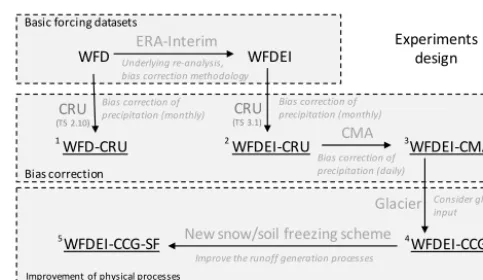
Figure 2.The flowchart of the five experiments designed for driv-ing the ORCHIDEE in this study. WFD and WFDEI are two basic forcing datasets. The underlined terms with numbers are the five ex-periments, while the grey arrows represent the development of the forcing compared to their previous ones.

3.2.1 Evapotranspiration simulation

On top of precipitation, evapotranspiration and potential evapotranspiration are two important fluxes, and their er-rors are key to the water cycle modeling. In ORCHIDEE, the evapotranspiration is calculated with energy balance and resistance concepts. The potential evapotranspiration is de-fined as “the amount of evapotranspiration that would occur if enough water was available at the surface”, as explained in Barella-Ortiz et al. (2013). The PET is computed as the sum of the potential soil evaporation and the potential tran-spiration from vegetation. For soil evaporation, the diffusive equations are taken with the ratio of the humidity gradient, the aerodynamic resistance and the air density. The virtual surface temperature is used instead of the actual one to com-pute the saturate humidity, while the virtual surface temper-ature is calculated through an unstressed surface energy bal-ance. The method has been proven superior to other diffusive methods in the reference paper Barella-Ortiz et al. (2013). The potential transpiration is driven by the potential evapo-ration between the evaporating surface and the overlying air but is limited by vegetation resistances. The maximal water loss under stress-free conditions is the potential transpiration (Guimberteau et al., 2012). The actual evapotranspiration is a function of the potential evaporation but is modeled by a se-ries of resistances (canopy and aerodynamics) of the surface layer. The details of the methods in simulating PET and ET can be found in D’Orgeval (2006), Guimberteau et al. (2012) and Barella-Ortiz et al. (2013).

3.2.2 Snow and soil freezing scheme

land area (Wang et al., 2013), and the frozen soils occupy 55 % to 60 % of the land surface of the Northern Hemisphere in winter (Zhang et al., 2003). Snow plays an important role in both the energy and water flux as the snow cover is first an insulation which prevents the heat loss from the soil. It also increases the thermal inertia of the surface by adding a new phase change and acts as a moisture reservoir which stores winter precipitation that is released in spring or early summer. In the old ORCHIDEE version, a constant density and very simple heat capacity are applied for the snow. The snowmelt directly feeds the runoff without refreezing, and the snow layer is mixed with the first soil layer so that they are equal in temperature. While in the new snow scheme, the snow layer is defined and separated from the soil layers. The snowpack is represented in three layers which adequately re-solve the snow thermal gradients between the top and base of the snow cover. The energy balance and the temperature of the snow body become more realistic. Refreezing of the snowmelt is allowed, which makes the energy changes more reliable. The snow properties are more detailed than before, i.e., the density, albedo and roughness. All the improvements have been validated over France and northern Eurasia and al-ready implemented in the current ORCHIDEE (Wang et al., 2013).

Soil freezing impedes water infiltration and drainage, thus leading to changes in hydrological responses (Woo and Marsh, 2005). At small scales, the soil freezing alters the soil structure and therefore its water capacity, which has a consequence on the water flux between soil and atmosphere, as well as the water availability for plants (Pitman et al., 1999; Huang et al., 2018). On the other hand, the frozen soil changes the latent heat exchange, which delays the soil tem-perature signal (Boike et al., 1998). Soil thermal characteris-tics are also improved due to the different thermal properties of ice and water. In the old soil thermal equations, thermal advection and phase change of the water are not considered when resolving the latent heat exchanges (Gouttevin et al., 2012). The mechanical effects of soil freezing are therefore ignored. In the new soil freezing scheme, the apparent soil heat capacity can be increased by considering the ice con-tent of the soil layer during a freezing-temperature window between 0 and −2◦C. A temperature correction is applied if any soil layer is entirely frozen or thawed. Moreover, the soil heat conductivity is changeable according to the ice con-tent in the soil, which affects the thermal propagation in the vertical soil column. Finally, the hydraulic conductivity is reduced as a function of the ice content. Liquid water is not allowed to cross the frozen soil layers. Thus infiltration and drainage are forced to stop. Full descriptions of the new freezing soil equations and the parameterizations setting can be found in Gouttevin et al. (2012).

3.2.3 Human intervention

Irrigation is included in the current version of ORCHIDEE. The irrigation requirement is estimated as the deficit of the available water of the corresponding grid to the potential evapotranspiration. The irrigation extracts water from the local grid first and then its neighboring grids if necessary (Guimberteau et al., 2012). This solution is acceptable for most of the humid regions at a 0.5◦resolution since the rivers are very likely within 100 km. However, for dry regions, the Tarim for example, the irrigation area is concentrated, with controlled irrigation infrastructures. The nearby rivers are far from the irrigation area, and the irrigated water is not taken directly from the rivers but transported from upstream by channels. Due to the shortcoming of the scheme and the lack of knowledge on the local irrigation, we turned off the ir-rigation in ORCHIDEE. In the Tarim Basin, the irir-rigation accounts for more than 95 % of the consumed water (Zhou et al., 2000), so that the difference between the simulated discharge and observations can be attributed to neglecting ir-rigation in the model.

In conclusion, as shown in Fig. 2, four different forc-ing inputs are prepared to drive the ORCHIDEE simula-tions, two basic forcing datasets (WFD-CRU and WFDEI-CRU), one after correction by CMA (WFDEI-CMA) and then one after adding glacier melt (WFDEI-CCG). Among them, the input water amounts are different, while WFDEI-CMA and WFDEI-CCG have the same other forcing vari-ables as WFDEI-CRU. Additionally, the experiment with the newly developed snow and soil freezing scheme is named WFDEI-CCG-SF based on the forcing dataset WFDEI-CCG. Because the WFD covers the overlapping period 1901–2002, the WFDEI covers the period 1979–2014, CMA covers years 1951–2016 and the glacier melt dataset covers 1958–2001, all the simulations and analysis in this paper are over the overlap period 1979–2001. The monthly discharge measure-ments for those chosen hydrological gauges over 1979–2001 are then compiled. Spatial resolution for all the forcing in-puts remains 0.5◦(about 50 km at the Equator), and the time step is 3 h.

3.3.1 Bias in precipitation

The Tarim Basin is one of the areas where significant devi-ations exist among different modeled precipitation estimates and observation-derived datasets because of the sparse obser-vations and orographic effects (Fekete et al., 2004; Wu et al., 2012). Meanwhile, the precipitation bias might not be well addressed in the CMA system because the number of mete-orological gauges is still too limited in the Tarim region to build a reliable interpolation climate field (Shen et al., 2010). Although Xie et al. (2007) have tried to use other gauges out-side China, the density of the gauge distribution is extremely low around the boundaries of the Tarim Basin where most of the precipitation is generated. Furthermore, due to the oro-graphic effects, the precipitation over the mountainous area is larger and with more significant heterogeneity than that in the plains (Daly et al., 2008; Barry and Chorley, 2009; Shi et al., 2017), while the center of the precipitation events is hard to observe for the nearby gauges. Adam et al. (2006) has pointed out that the orography could cause 41.6 % under-estimation of the precipitation over the northwestern North American mountainous ranges, and the deviations are larger at higher altitude.

3.3.2 Bias in rainfall and snowfall repartition

The differences between WFDEI-CRU and WFDEI-CMA are not only in the total amount of precipitation but also in the proportion of rainfall and snowfall (Table 3). Compared to the rainfall, the snowfall is more difficult to observe and affected by a large uncertainty; hence in the CMA dataset, only the rainfall was recorded and then used to scale the CRU dataset but keeping the relative proportion of liquid and solid precipitation provided by WFDEI-CRU. The energy needs for phrases change are considerably different for the liquid from the solid water. Berghuijs et al. (2014) suggested snow will lead to more runoff than rain in similar conditions based on the observations over the US and China. The impact of the precipitation type on the evapotranspiration rate is affected by many factors and hard to measure.

3.3.3 Bias in glacier melt

HYOGA2 is a state-of-the-art global glacier model but has not been calibrated over the Tarim Basin. The general bias for global estimation is around −5.0 % compared to the avail-able global glacier mass balance measurements (Hirabayashi et al., 2013). The estimated annual glacier melt amount is 81.0×108m3yr−1 for the whole Tarim Basin (Table 3), significantly lower than previous estimations (Yang, 1991: 133.4×108m3yr−1; Gao et al., 2010: 144.16×108m3yr−1). On the one hand, the difference in the forcing which drives the glacier melting model is probably one of the causes of the deviation. On the other hand, all the glacier melt is evenly distributed in a whole grid. It leads to a higher infiltration

ra-tio and thus feeds more evaporara-tion (Berger and Entekhabi, 2001; Potter et al., 2005). This also artificially forces part of the glacier melt to flow out of the grid not belonging to the right basin. However, it is unable to eliminate this problem with the current gridded concepts. Finer spatial resolution in glacier dataset and model simulation is needed to lessen the impacts of discretization.

3.3.4 Bias in potential evapotranspiration estimation As described in Sect. 3.2.1, the PET estimation is indepen-dent of underlying conditions (e.g., topography, vegetation) because enough water is provided. It is therefore determined only by forcing conditions, especially the humidity gradient and aerodynamic conditions (e.g., radiation flux, wind). Tem-perature also plays a role in its estimation. Thus, the bias in PET is mainly propagated from various forcing variables.

3.3.5 Bias in actual evapotranspiration estimation Overestimation (underestimation) of the actual ET will also result in the discharge underestimation (overestimation). Many processes can cause ET errors either by the biases in PET or the stress functions which limit the potential evapora-tion. The vegetation fraction, vegetation type, surface slope and soil properties are all the uncertain sources affecting the final ET estimation.

3.3.6 Bias sources category

With the main biases listed as above, we consider bias in any processes that changesP or PET as bias from forcing and bias in any processes that directly changes ET as bias caused by model structure. Although the shifts in forcing variables will change the ET estimation – for example, the

P restricts the available water for ET – this shift still belongs to the forcing category since the relation is indirect. The bi-ases which directly affect ET include bibi-ases in infiltration, soil water movement, snow processes, vegetation representa-tion and many other model processes. And all these are con-sidered as biases caused by model structures.

3.4 Budyko hypothesis

Table 1.Different formulas of Budyko curves. Note that the aridity index is expressed as∅=PET/ P.

No. Parameter Formula Reference

1 Non-parameter ET/P=1−e(−∅) _{Schreiber (1904)}

2 Non-parameter ET/P=_∅tanh(1/∅) Ol’dekop (1911)

3 Non-parameter ET/P=1/(1+(1/∅)2)0.5 Pike (1964) 4 Non-parameter ET/P= {[1−e−∅] ·_∅·tanh(1/∅)}0.5 Budyko (1974)

5 Parametern ET/P=1/[1+(1/∅)n]1/n Mezentsev (1955); Choudhury (1999); Yang et al. (2008)

6 Parameter$ ET/P=1+_∅− [1+(∅)$]1/$ Fu (1981) 7 Parameter$ ET/P=(1+$∅)/(1+$∅+1/∅) Zhang et al. (2001)

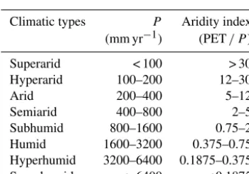
Table 2.The definition of climate types by precipitation and aridity index (Ponce et al., 2000).

Climatic types P Aridity index

(mm yr−1) (PET/ P)

Superarid < 100 > 30

Hyperarid 100–200 12–30

Arid 200–400 5–12

Semiarid 400–800 2–5

Subhumid 800–1600 0.75–2

Humid 1600–3200 0.375–0.75

Hyperhumid 3200–6400 0.1875–0.375

Superhumid > 6400 < 0.1875

The forms without parameters (formulas 1 to 4) are univer-sal for most of the basins, while they are unable to capture the various landscape characteristics across regions (Yang et al., 2007). Regarding the effects of landscape characteristics, ad-justable parameters and corresponding formulas were intro-duced as formula (5) to (8). Although they have different ana-lytical expressions, the shape of these curves is quite similar (Gerrits et al., 2009) and their parameters are highly corre-lated (Yang et al., 2008). Hence, from the formulas with pa-rameters, Fu’s equation (formula 6) is chosen in this study as it is more often used in the China region.

The ranges of the aridity index (PET/ P) correspond to the regional precipitation feeds and climate types (Table 2). For example, the precipitation for a semiarid region ranges from 400 to 800 mm yr−1, and the regional aridity index mostly ranges from 2 to 5. Moreover, the Budyko curve is a reflection of the landscape characteristics which can influ-ence the water movement through different hydrological cy-cles (Dingman, 2015) and thus changes the ET rate. Many surface conditions are related to the Budyko parameter set-ting. (1) Vegetation types and vegetation cover affect the ET rate. Transpiration accounts for about 42 % (25 %–64 % de-pends on different models) of global ET (Zhang et al., 2004). Regions that have a larger fraction of vegetation cover or are covered by vegetation with bigger leaves and deeper roots tend to have a larger transpiration rate as well as ET rate;

i.e., the forested catchment tends to show a higher evapora-tion ratio than the grass-covered catchments (Zhang et al., 2004; Carmona et al., 2014). (2) Properties of soil determine infiltration rates and the amount of evapotranspirable water. Steeper slopes are more likely to shed surface water as runoff (Yang et al., 2007; Yu et al., 2014). Limit of infiltration abil-ity also matters as intense precipitation rates (Berger and En-tekhabi, 2001; Potter et al., 2005) or freezing soils tend to force the water into the surface runoff (the solid frozen soil limits the percolation of infiltrated water; Gouttevin et al., 2012). (3) The ability to transmit or retain infiltrated water of soil also determines the evapotranspiration rate; the soil with larger water conductivity is likely to release more sub-surface water rather than evaporation (Yang et al., 2007). (4) The soil depth determines the ability to store infiltrated water. Rocky mountains or regions with thin soil would pro-duce more runoff and less ET (Yang et al., 2008; Dingman, 2015).

3.5 Bias assessment with the ORCHIDEE-Budyko framework

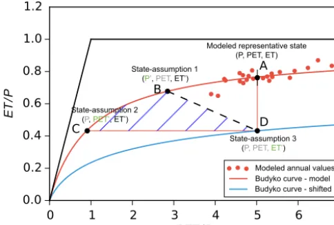
The Budyko formulation relates the ET to PET andP. Both the biases from the water flux (P) and energy flux (PET) will propagate to ET. The shape parameter of the Budyko curve is obtained by fitting the PET/ Pand ET/ P relation; it is thus a reflection of the model if we use the simulated PET and ET fluxes (i.e., ORCHIDEE simulations in this study, red dots and red curve in Fig. 3). However, because of the existing bias in all the three variables, the relations of the three com-ponents may have been shifted to an unrealistic state (point A in Fig. 3). Therefore, the changes inP, PET or ET which can shift the system back to a reliable state are considered as the possible bias. The difference between the unrealistic state with their corrected values provides the estimation of how the forcing or the model would need to be changed for the model to produce the realistic discharge values. To separate the in-dividual effect of the single water–energy component on the hydrologic cycle, three independent assumptions are made as follows, and the illustration can be found in Fig. 3.

The red dots in Fig. 3 represent the states of the PET/ P

forc-Budyko curve - model Budyko curve - shifted Modeled annual values Modeled representative state

(P, PET, ET)

PET/P

E

T

/P

State-assumption 1

(P’, PET, ET’)

State-assumption 2

(P, PET’, ET’)

State-assumption 3

(P, PET, ET’)

Figure 3.The illustration of the ORCHIDEE-Budyko framework. Point A represents the average state among the modeled annual val-ues (with the land surface model ORCHIDEE), and the red curve is the simulated Budyko curve following the modeled state. Points B, C and D represent the representative state with theP, PET and ET shifted, respectively, with different assumptions to meet the discharge observations. A shifted Budyko curve (blue) is obtained crossing the point D, which indicates a new state of the model struc-ture. The new points of B and C still stay on the original Budyko curve, indicating that the model structure remains the same and the changes only relate to forcing variables. The shaded area is the area among the three shifted states.

ing inputs for each year. Point A represents the representative state, which is the average of the dots’ locations. It reflects the current model and is probably in an unrealistic state be-cause the modeled discharge (P−ET) may be with bias com-pared to the observations.

Assumption 1. Only the water input (P) is uncertain. Because the model structure remains unchanged, the rela-tion between ET/ P and PET/ P still follows the original Budyko line regardless of how P changes. The PET is as-sumed to be independent ofP, while the ET is modified as a result ofP changes. To meet the deviation between simu-lated discharge (RS) and the observed discharge (RO), the representative point (long-term “corrected” annual ET/ P

against long-term “corrected” annual PET/ P) should be shifted along the Budyko curve from current point “A” to the new point “B”, where the difference between the “true” pre-cipitation (P0) and the “true” evapotranspiration (ET0) equals the observed discharge (P0−ET0=RO). The possible max-imum bias inP is calculated as

bias(P )=(P−P0)/P0×100 %. (1)

Assumption 2.Only the PET is uncertain. TheP remains the same, while ET changes because of the changes in PET. Under these conditions, the model structure still remains un-changed, and so does the Budyko curve. Then the representa-tive point should be shifted along the Budyko curve to point “C” to decrease the ET ratio to meet the discharge

observa-tion (ET0=P-RO). The PET is changed to a “true” PET0, and the possible maximum bias in PET is calculated as bias(PET)=(PET−PET0)/PET0×100 %. (2)

Assumption 3.Only the ET is uncertain.P and PET, which are mainly linked to the forcing, remain the same, while the ET, which is significantly affected by the model structure, is assumed biased. It is essentially relevant to the model pro-cesses rather than the forcing dataset. To compensate the discharge bias, the ET should be decreased to point “D” where the ET equals precipitation minus observed discharge (ET’=P−RO). The possible maximum bias in ET is calcu-lated as

bias(ET)=(ET−ET0)/ET0×100 %. (3) With the target ET0, a new Budyko curve can be drawn for new relations betweenP, PET and the new ET (the blue lines in Fig. 3). However, all the assumptions are proposed in con-ditions of only one variable being uncertain, but in reality any of the three variables can be biased at the same time. The final probable “corrected” state may be located in the shaded area identified by the three states (Fig. 3).

4 Results and discussion

4.1 Forcing and discharge comparison

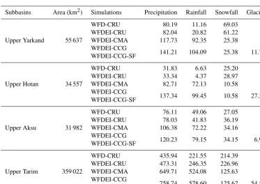
4.1.1 Forcing input comparison among experiments We specifyP as the sum of all the water inputs into the sys-tem, which include the atmospheric water flux (in its liquid and solid phases) and glacier melt. The precipitation for the three headwater catchments and the upper Tarim is listed in Table 3 for each simulation. The interannual variations and the intra-annual cycle of total precipitation over upper Tarim Basin are plotted for different forcing in Fig. 4.

(a) _-1 (b)

-1

-1

-1

Figure 4.The interannual cycle and intra-annual series of the precipitation (including rainfall, snowfall and glacier) in difference simulations for the upper Tarim Basin.

Table 3.The five simulations in this study and basic diagnostics of the water inputs over three headwater catchments and the upper Tarim Basin. Units: 108m3yr−1.

Subbasins Area (km2) Simulations Precipitation Rainfall Snowfall Glacier

Upper Yarkand 55 637

WFD-CRU 80.19 11.16 69.03 –

WFDEI-CRU 82.04 20.82 61.22 –

WFDEI-CMA 117.73 92.35 25.38 –

WFDEI-CCG

141.21 104.09 25.38 11.74

WFDEI-CCG-SF

Upper Hotan 34 557

WFD-CRU 31.83 6.63 25.20 –

WFDEI-CRU 33.34 4.37 28.97 –

WFDEI-CMA 82.71 72.13 10.58 –

WFDEI-CCG

137.34 99.45 10.58 27.31

WFDEI-CCG-SF

Upper Aksu 31 982

WFD-CRU 76.11 49.06 27.05 –

WFDEI-CRU 78.03 41.83 36.19 –

WFDEI-CMA 106.38 72.22 34.16 –

WFDEI-CCG

120.23 79.15 34.15 6.93

WFDEI-CCG-SF

Upper Tarim 359 022

WFD-CRU 435.94 221.55 214.39 –

WFDEI-CRU 473.31 246.35 226.96 –

WFDEI-CMA 649.71 524.08 125.63 –

WFDEI-CCG

758.74 578.60 125.62 54.52

WFDEI-CCG-SF

in CMA, to which the decrease in snowfall is the major con-tributor. The changes in rainfall and snowfall are similar in all three headwater catchments (Table 3) and the upper Tarim Basin.

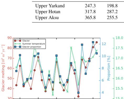
Adding the glacier melt leads to negligible changes dur-ing winter and sprdur-ing but large increases in the total water inputs in summer (JJA) when the temperature is higher. The estimated glacier melt is 9.1 %, 25.8 % and 6.1 % to the total water inputs for the upper Yarkand River, upper Hotan River and upper Aksu River. It significantly increases after 1990 (Fig. 5; the trend is +3.8×108m3yr2, p=0.024), being consistent with its ratio to the total water input (r=0.918,

p <0.001). The trend is mainly caused by climate warming

as the glacier melt is highly correlated with the summer tem-perature (r=0.852, p <0.001). The increasing trend has also been documented in glacier runoff observations (Shang-guan et al., 2009).

4.1.2 Assessment of the discharge estimations with observations

In-Table 4.The water–energy components for the headwater catchments in WFDEI-CCG-SF simulation. Units: mm yr−1.

Precipitation Rainfall Snowfall Glacier ET RS PET RO

Upper Yarkand 247.3 198.8 48.5 22.4 188.3 59.1 1240.4 140.4

Upper Hotan 317.8 287.2 30.6 78.9 236.9 81.3 1153.7 118.9

Upper Aksu 365.8 255.5 110.3 22.4 238.1 128.0 631.8 250.1

-1

Figure 5.The temporal variations of the glacier melt, the proportion of glacier melt in the water input and the average summer temper-ature over the upper Tarim Basin. They are in good correlation and have a consistent increasing trend after 1990.

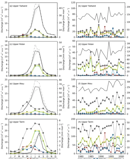
stead, the discharge measurement can serve as a better ref-erence since it integrates the net water flux over the entire basin. Therefore, driven by the forcing, ORCHIDEE was used to simulate the river discharge and for comparison to in situ observations (Fig. 6). The corresponding assessment using criteria for the three headwater catchments are plotted in Fig. 7. For the three headwater catchments where most of the discharge of the Tarim Basin is generated, the discharge is significantly underestimated, with the underestimation ra-tio reaching 90 % (Figs. 6b, d, f, 7a) for CRU datasets. Dis-charge increases after the precipitation is corrected by the CMA dataset, with the absolute bias decreasing to around 80 %. Adding glacier melt also increases the discharge but by a relatively small amount. Changes in the model struc-ture (new snow and soil freezing scheme) further decrease the bias, especially for the Aksu River. The final biases of the discharge for the three subbasins are−71.1 %,−47.8 % and−49.4 %. The gradual improvements and corresponding magnitude changes are visible in the annual discharge vari-ability in Fig. 6b, d and f.

Besides the increase in the annual mean discharge, the am-plitude of the interannual cycle of the discharge is also im-proved by the progressive changes. The estimated discharge peaks have been shifted from April in CRU simulations to the summer (July or August) by CMA correction and adding glaciers (Fig. 6a, c, e). Correspondingly, the correlation of the annual variability between the estimated and observed discharge has increased above 0.9 for all the three subbasins with the WFDEI-CCG forcing (Fig. 7b). However, contrary

to the upper Yarkand River and the upper Hotan River, the introduction of the new snow and soil freezing scheme de-creases the discharge correlation for the upper Aksu River from 0.91 to 0.42. An early discharge peak exists in May, while not enough runoff is generated in the summer period (Fig. 6e). Although the correlation decreases, it does not mean the model/simulation deteriorates because correlation only evaluates the similarity of temporal variation but ignores the fact that the discharge amount has been better estimated (Figs. 6e and 7a).

By extracting the observed discharge in the first and last 5 years from the whole period, we can notice there is an obvious shift of the discharge peak from August to July in the three headwater catchments (Fig. 6a, c, e). The regional precipitation changes largely cause the shift, but the increas-ing temperature also allows the snow/glacier to melt at a higher rate in the most recent period. Furthermore, increas-ing trends are detected after the 1990s (Fig. 6b, d, f), as the increasing trend is 1.43×108m3yr2(or 0.77×108m3yr2, 1.78×108m3yr2) for the upper Yarkand (or Hotan, Aksu) River. The increasing trends are consistent with the glacier melt, glacier proportion in water input and summer tempera-ture in the same period (Fig. 5).

The trends in the estimated discharge are also calculated and compared with the observed trends, expressed as the ra-tio of the trend in estimara-tion to that in observara-tions (Fig. 7c). For CRU simulations, no increasing trend is detected since the ratio is less than 0. The CMA correction increases the ra-tio for all three subbasins to around 0.3, which means the pre-cipitation accounts for only around 30 % of the discharge in-crease. Adding the glacier melt increases the ratio from 0.35 to 0.54 for the upper Hotan River and from 0.31 to 0.76 for the upper Aksu River; the improvement of the glacier melt-ing is comparable to the CMA correction. However, no ap-parent changes are detected for the upper Yarkand River. By comparing the criteria between CMA and WFDEI-CCG, we find that, although adding the glacier melt does not change much the absolute amount of discharge or the correla-tion, the increased trend in discharge has been considerably improved. The increasing glacier melt is, therefore, one of the contributors to the discharge trend in the Tarim. The mod-ification of the snow and soil freezing scheme increases the trend ratio in the upper Aksu River up to 0.72, while slightly decreasing it for the two other catchments.

(a) Upper Yarkand (b) Upper Yarkand

(c) Upper Hotan (d) Upper Hotan

(f) Upper Aksu

(g) Upper Tarim (e) Upper Aksu

(h) Upper Tarim

-1

-1

-1

-1

-1

-1

-1

-1 -1

-1

-1 _-1

-1

-1

-1

-1

Figure 6.The interannual cycle and intra-annual series of the discharge simulation for three headwater catchments and the upper Tarim Basin:(a, b)Yarkand River,(c, d)Hotan River,(e, f)Aksu River and(g, h)the upper Tarim Basin. Observed discharge for each subbasin was aggregated by the measurements at separated discharge gauges and shown as the black solid line. The simulated discharges at the corresponding grids were extracted from each experiment and plotted as the color lines with markers. The dotted line and dot-dash line in the interannual cycle plots represent the observed discharge in different periods.

WFDEI-CCG) is effective for improving the model perfor-mance using different criteria (bias, correlation, proportion to the trend) to compare the observed discharge. The three criteria are independent as they stand for the averages, the

Table 5.The annual average values for different water–energy components (P, ET, PET; units: mm yr−1) and their relations (P−ET, PET/ P

and ET/ P) for the three upstream subbasins. The scenarios correspond to the diagnostics of the current model (A) and three bias assumptions listed above from B to D. The bold values are the main factors changed within the three basic water–energy components. The changing ratio indicates the ratio of the changing value to the original value (unit: %), while the bias range implies the bias of the values in the current variables compared to the values they should be (unit: %).

P PET ET P−ET PET/ P ET/ P Factor Changing ratio Bias range

Upper Yarkand

A 247.3 1240.4 188.3 59.0 5.02 0.76 – –

-B 435.4 1240.4 294.9 140.5 2.85 0.68 P 76.1 % −43.2 %

C 247.3 225.0 106.9 140.4 0.91 0.43 PET −81.9 % 451.2 %

D 247.3 1240.4 106.9 140.4 5.02 0.43 ET −43.2 % 76.1 %

Upper Hotan

A 317.8 1153.7 236.9 80.9 3.63 0.75 – – –

B 402.3 1153.7 283.3 119.0 2.85 0.70 P 26.6 % −21.0 %

C 317.8 615.2 198.8 118.9 1.94 0.63 PET −46.7 % 87.5 %

D 317.8 1153.7 198.8 118.9 3.63 0.63 ET −16.1 % 19.1 %

Upper Aksu

A 365.8 631.8 238.1 127.7 1.73 0.65 – – –

B 553.3 631.8 303.1 250.2 1.14 0.55 P 51.3 % −33.9 %

C 365.8 174.1 115.7 250.1 0.48 0.32 PET −72.4 % 262.4 %

D 365.8 631.8 115.7 250.1 1.73 0.32 ET −51.4 % 105.8 %

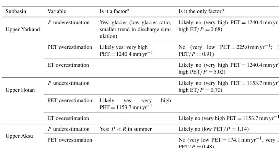
Table 6.Summary of the possible causes of the underestimation in discharge and the corresponding arguments. Three levels of the possibility are presented: yes: with direct argument; likely: with indirect argument; and no: with negative argument.

Subbasin Variable Is it a factor? Is it the only factor?

Upper Yarkand

P underestimation Yes: glacier (low glacier ratio, smaller trend in discharge sim-ulation)

Likely no (very high PET=1240.4 mm yr−1; high ET/P=0.68)

PET overestimation Likely yes: very high PET=1240.4 mm yr−1

No (very low PET=225.0 mm yr−1; low PET/P=0.91)

ET overestimation Likely no (very high PET=1240.4 mm yr−1;

high PET/P=5.02)

Upper Hotan

P underestimation Likely no (very high PET=1153.7 mm yr−1;

high ET/P=0.70)

PET overestimation Likely yes: very high PET=1153.7 mm yr−1

ET overestimation Likely no (very high PET=1153.7 mm yr−1)

Upper Aksu

P underestimation Yes:P < Rin summer Likely no (low PET/P=1.14)

PET overestimation No (very low PET=174.1 mm yr−1, very low

PET/P=0.48)

ET overestimation

the most significant improvement to all the criteria. The role of glaciers melting is critical for the trend analysis. The mod-ification in the snow and soil freezing scheme increases the total discharge amount but could lead to adverse responses in the correlation and trend simulation. However, the impact of the modification of the model structure is not larger than changes resulting from the forcing biases. From the previous analysis, we can conclude that the simulations of

(a) (b) (c)

Figure 7.The discharge diagnostics of different experiments for three catchments (round – Yarkand; square – Hotan; and triangle – Aksu).

(a)represents the absolute bias in percentage, (b)represents the correlation of the interannual cycle and(c)represents the ratio of the trend in estimated discharge to that in observed discharge for the period 1990–2001. S0 to S4 correspond to the experiments WFD-CRU, WFDEI-CRU, WFDEI-CMA, WFDEI-CCG and WFDEI-CCG-SF in ascending order.

(a) (b)

(c) (d)

(e) (f)

-1

-1

-1

-1

-1

-1 -1

-1

-1 -1

-1

-1

(a) (b)

(c)

Figure 9.Budyko relation for three headwater catchments (a, Yarkand;b, Hotan;cAksu). The red points represent the values for each year; thePis obtained from the forcing, while ET and PET are obtained from the model. Point A represents the long-term average Budyko relation, and red lines are the optimal fitted Budyko line. The water inputP, the potential evapotranspiration PET or the actual evapotranspiration ET can be modified to meet the observed discharge, which correspondingly shifts the representative points from A to B, C or D. B and C stay in the original Budyko curve, while a new optimal fitted Budyko curve through point D can be built after the changes in ET. The shaded area is the most likely area when not only a single variable is changing.

4.2 Evidence of the bias in estimated discharge for the headwater catchments

Although the simulations with WFDEI-CCG-SF are better than other experiments, there are still biases compared to the observations (Fig. 7a). In this section, we aim to find evi-dence of the biases. The annual mean water balance compo-nents (rainfall, snowfall, glacier melt, estimated ET and dis-charge RS) of the three upper catchments are plotted as bars with their relations quantified by comparison to the discharge observations (RO, red lines in Fig. 8a, c, e) in WFDEI-CCG-SF. Their annual cycles are also plotted as Fig. 8b, d and f over the three headwater catchments. Over a long enough period, the changes in terrestrial water storage are assumed negligible compared to the water fluxes, so that the water in-put into the system either returns to the atmosphere through ET or flows out of the basin as RS.

From the left panels of the Fig. 8, we have a visual im-pression of the relative amount of different water inputs and their contribution to the ET or discharge. Note that the sum of the ET and RS is not exactly equal toP because in OR-CHIDEE the discharge is represented at the outflow of the grid and not at the confluence point of the analyzed catch-ment with other tributaries. The largest bias is 8 % for the up-per Yarkand River (Fig. 8a, ET/ P+RS/P =0.92), while

it matches exactly for the upper Aksu River. The bias can be added to the current RS if necessary.

Among the three headwater catchments, the upper Hotan River has the best discharge simulation compared to the ob-servations (RS/RO=0.52). The annual cycle of the water also matches well as all theP, ET and discharge RO or RS have the synchronous peaks in summer (Fig. 8d). There are also deviations betweenP andE, which represent the net water inputs to the system and the estimated discharge (the shaded area with blue lines in Fig. 8d). The deviation implies the regional water storage changes; in summer the soil mois-ture increases to store the abundant water inputs, which are later released in autumn and winter when the drainage rate is larger than infiltration. The water storage decreases as a result by then. It is the natural adjustment to the strong sea-sonality in water inputs.

The upper Aksu River has different characteristics from the other two regions since it lies in the northern part of the Tarim. It has a larger snowfall proportion in the precipitation. Meanwhile, it has the largest ratio of estimated ET/PET, the largest runoff generation ratio (RS/P =0.35) and the least discharge simulation error (RS/RO=0.51). However, there is certainly large bias in the regional precipitation as the dis-charge has exceeded the precipitation input in the summer period (July and August). The estimated annual cycle of dis-charge diverges from the observations (Fig. 8f), as its peak advances by 2 months and the discharge estimation signifi-cantly exceeds the observations in spring (MAM). The runoff generation ratio in the summer period is also unrealistically low.

In summary, the biases in discharge estimation exist in terms of the total amount and the annual cycle. Precipita-tion is one of the largest bias sources, which makes the bias analysis in models more difficult.

4.3 Bias range and possibility analysis for the headwater catchments

Although either P or PET or ET can cause final underes-timation of discharge over the three headwater catchments, quantifying the bias in each flux is challenging and imprac-tical due to the lack of direct measurements and the strong heterogeneity over the mountainous area. To separate the in-dividual bias, we use the Budyko hypothesis by assuming only one variable is uncertain, while the other two are as-sumed to have negligible errors, with which we “correct” the model simulation to meet the discharge observation and ob-tain the possible bias range. Then we evaluate the possibility of rejecting the assumption to find the most likely bias source by checking the status of the water system (i.e., amount of the water–energy components and their relations) in indi-rect ways. The water–energy components used in the Budyko analysis are all ORCHIDEE outputs of the most satisfactory simulation, WFDEI-CCG-SF. The corresponding character-istics of the water–energy components for three headwater catchments are listed in Table 4.

4.3.1 Bias ranges estimated by the ORCHIDEE-Budyko framework

The ORCHIDEE-estimated evapotranspiration rate (ET/ P) against the estimated aridity index (PET/ P) over each sub-basin in each year is scattered as red points in Fig. 9. Point A represents the Budyko relation between long-term average annual ET/ P and the long-term average annual PET/ P. According to the categories introduced by Ponce et al. (2000), all three catchments belong to semiarid climate zones by the definition of the annual average precipitation (Table 2). Hence the aridity index is supposed to range from 2 to 5. Regarding the high elevation and cold temperature, the PET rate is likely to be smaller than the representative

climate of this aridity index. Thus the aridity index for the three catchments is supposed to be lower than expected. It is realistic for the upper Hotan River and the upper Aksu River as their aridity is 3.63 and 1.73, respectively. While the arid-ity index for the upper Yarkand River is 5.02, which can be categorized as a semiarid or arid region, this is not very likely since the upper Yarkand River is providing water resources for the irrigated area over the lower Yarkand oases (Zhou et al., 2000; Mamitimin et al., 2014).

However, because there is still a bias in the ORCHIDEE discharge estimations with the observations, the current state A is not correct. Based on the assumptions introduced in Sect. 3.5, the three possible “corrected” states by shifting the

P, PET and ET are shown in Fig. 9 for the three headwater catchments. Taking the upper Yarkand River as an example (Fig. 9a), if we consider onlyP to be biased (assumption 1), theP has to be shifted from 247.3 to 435.4 mm yr−1_{. PET} mains the same, and the ET changes accordingly, but the re-lation between ET/ P and PET/ P still follows the Budyko curve. The state is shifted from point A to point B with the

P change ratio as 76.1 %. Reversely, the possible bias of

P is−43.2 % ((247.3–435.4)/435.4×100 %). Similarly, to change the PET in order to shift the state to correct (point C, assumption 2), the PET has to be shifted from 1240.4 to 225.0 mm yr−1. The possible bias in PET is 451.2 %. To change the ET in order to shift the state to correct (point D, assumption 3), the ET has to be shifted from 188.3 to 106.9 mm yr−1, and the possible bias in ET is 76.1 %. The route is the same for the other two catchments, and their re-sults are listed in Table 5.

The previous analysis is based on the assumptions that theP and PET are independent and only a single variable is uncertain, which might be invalid in reality. However, the three assumptions provide the bias boundaries of each vari-able, and the final system reproducing observed RO is likely to be located within the shaded area shown in Fig. 9. Tak-ing the Hotan River as an example, to meet the discharge observation, the final changes inP will be 0 %–26.6 %, the decrease in PET will be 0 %–46.7 % and the decrease in ET will range 0 %–16.1 %. While in turn, we also conclude that theP is underestimated by 0 %–21.0 %, the PET is overes-timated by 87.5 % at most and the ET is overesoveres-timated by 19.1 % at most. If we know the bias for any single variable, the feasible ranges will be narrower than at present.

4.3.2 Ranking the bias possibility

From multiple-model analysis based on CMIP5 general circulation models (GCMs), the estimated PET over the western boundary of the Tarim Basin is about the same as over the Tibetan Plateau (Scheff and Frierson, 2015). How-ever, because of the unpredictable biases in GCMs, the ab-solute values are not highly reliable in their simulation. Nev-ertheless, the equivalent relation provides us with the ranges of PET over the Tarim headwater catchments by referring to the observations over the Tibetan Plateau, where the to-pography changes are relatively small and the observations are more abundant. According to Chen et al. (2006), who used site observations from 101 stations over the Tibetan Plateau, the annual average PET over the plateau ranges from 580 to 720 mm yr−1. Hence the PET over the upper Yarkand River and the upper Hotan River is probably overestimated (1240.4 and 1153.7 mm yr−1). Therefore, only changes inP

or ET are not satisfactory because the PET is unchanged. For the upper Yarkand River, the PET is not the only error source, because, to match the discharge deviation by only de-creasing PET, the PET should be decreased to 225 mm yr−1, which exceeds the referenced PET range. Moreover, because Yarkand and Hotan are neighboring regions which have sim-ilar climates, the PET should be a simsim-ilar amount in each (615.2 mm yr−1if only PET is uncertain in the upper Hotan River, while 225 mm yr−1 in the Yarkand River). The esti-mated PET over the Aksu River is realistic since the PET is 631.8 mm yr−1for the current scenario, but it would de-crease to 174.1 mm yr−1if only the PET changed, which is too low. Besides the absolute value of PET, the ratio PET/ P

also shifts when PET changes, which means the climatic types can be changed. Only decreasing the PET in the upper Yarkand and the upper Aksu River would cause significant decreases in the aridity index (from 5.02 to 0.91 for the up-per Yarkand, from 1.73 to 0.48 for the upup-per Aksu River), which are not realistic for these regions.

ET computation is sensitive to the climatic conditions and the surface conditions; hence the absolute value of ET sig-nificantly varies in time and space, and its bias very diffi-cult to quantify. The evapotranspiration ratio to precipitation (ET/ P) is typical for specific climatic types or regions with similar land cover types (Yang et al., 2007). Liu et al. (2003) estimated the evapotranspiration ratio to precipitation using a remote-sensing approach over regions of Canada. They con-cluded that the ratio ET/ P is 32 % for barren land and 18 % for snow/ice land. In general, most of the catchment area of the three headwater catchments consists of barren and snow/ice land. Because of its lower latitude, the ET ratio could be higher but still below the rate for cropland (67 %). Therefore, only changes inP are not very likely for Yarkand and Hotan (ET/ P is 0.68 for Yarkand and 0.70 for Hotan after the correction). Higher P for the upper Aksu River is likely to maintain a realistic ET/ P ratio.

The biases of the three variables (P, ET, PET) have rela-tively weak dependence because they are governed by differ-ent processes.P and PET are quite independent because they

relate to different forcing variables. Although the ET amount is linked to two other variables, the ET bias is weakly de-pendent, and it also comes more from the surface conditions and model biases. The chances of biases arising from each variable are about the same in theory. However, based on the analysis of the model output and the assumed bias-corrected scenarios, there are some priorities for the bias sources over each subbasin. The possibility of biases and the supporting arguments are listed in Table 6 for each headwater catch-ment. For instance, for the upper Yarkand subbasin, an in-crease inP, especially the glacier melt, is necessary because of the lower glacier melt ratio compared to the Hotan basin (Sect. 5.1.2.3) and the small trend in model discharge com-pared to the discharge observation (Sect. 4.2). However, only increasing the precipitation is not sufficient because the cur-rent PET is very likely too high compared to the surround-ing regions (PET=1240.4 mm yr−1_{, while PET ranges 580–} 720 mm yr−1_{over the Tibetan Plateau). Meanwhile, only} de-creasing the PET without changing other variables would cause a very low PET rate (225 mm yr−1) and low aridity index (PET/P =0.91), which is not realistic for this region. Modification in ET is possible but not adequate due to the overestimated PET. Hence, this error analysis reveals that increasing precipitation over the upper Yarkand subbasin is quite necessary, the overestimation of PET is very likely and modification in ET estimation is possible but not fundamen-tally necessary. For the upper Hotan River, the most likely biases come from the overestimation of PET, while the two other variables are possible sources. An increase in precipi-tation and changes in temporal variability are necessary for the upper Aksu subbasin, but they are not the only causes, as either the PET or ET, or both, is overestimated.

4.4 Human intervention in the lower oases

The current ORCHIDEE version does not yet take into count the intensified evapotranspiration caused by human ac-tivities especially through irrigation, which is a major pro-cess in the hydrological cycle transferring water to the atmo-sphere. As a consequence, in the lower oases the simulated discharge at the Alar station is significantly larger than the observations (Fig. 6g, h; 146.59×108m3yr−1 in WFDEI-CCG-SF simulation to 43.34×108m3yr−1in observation). However, because the biases of the upstream discharge will propagate to the Alar station, the catchment of which in-cludes the three basins discussed above, the currently esti-mated discharge is thus underestiesti-mated compared to the po-tential river flow at Alar, which is the natural river flow with-out human intervention.

of discharge from those three catchments. The increment at Alar should be 110.25×108m3yr−1_{(observed 192.15×} 108m3yr−1_{from the three headwater catchments minus} sim-ulated 81.9×108m3yr−1), so that the potential river flow at Alar should be 256.84×108m3yr−1 (=146.59+110.25), and the influence of human activities on the increase of ET can be estimated as 213.50×108m3yr−1(=256.84−43.34), 83.1 % of discharge.

A second simple scaling approach to obtaining the poten-tial river flow at Alar is that we assume the model bias for the whole upper Tarim Basin is constant over space. The scaling factor is 2.35 (=192.15/81.9); hence the potential discharge at Alar should be 343.92×108m3yr−1(=146.59×2.35). And the influence of human activities on the increase of ET is es-timated as 300.58×108m3yr−1(=343.92−43.34), 87.4 % of the discharge. The overestimation over the discharge ob-servation is the amount caused by additional human interven-tion, especially the irrigation-caused evapotranspiration.

To validate the proposed values, we collected the irriga-tion area over the Tarim Basin using the FAO Global Map of Irrigation Areas (Siebert et al., 2013), according to which the total irrigated area for the upper Tarim Basin is 13 548.5 km2. In addition, Zhou et al. (2000) provides the gross irriga-tion quota as 1.77×106m3km−2; hence the total irriga-tion water consumpirriga-tion will be 239.80×108m3yr−1. Hence the results of the two approaches assessing human net ab-straction are −11 % and 25 % (213.50×108m3yr−1 and 300.58×108m3yr−1, respectively) in relation to the con-sumption data, which are acceptable figures because of the unknown biases in irrigation area as well as the gross irriga-tion quota. The proporirriga-tion of the consumed water (83.1 %– 87.4 %) is higher than the estimation (74.7 %) in 1995, which could be explained by the intra-annual variation of inflow and abstraction.

5 Conclusions

In this work, we proposed an ORCHIDEE-Budyko frame-work which is used to attribute the modeled discharge bias to different sources as the forcing and model structure. Bias in the precipitation (P) and any processes related to the po-tential evapotranspiration (PET) is considered as bias from forcing and bias in any processes affecting the actual evap-otranspiration (ET) estimation is considered as bias from model structures. The discharge simulation was provided by the land surface model ORCHIDEE with latest developments in its modules and driven by the most improved forcing in-puts (WFDEI-CCG-SF). However, underestimation in the discharge still exists over the three Tarim headwater catch-ments, where the biases ofP, PET and ET are analyzed with a Budyko analytical approach. With a set of assumptions, we isolated the biases in three variables, and their possibili-ties were assessed with information from nearby and hydro-climatically similar regions. Results show that precipitation

(here considered as the sum of rainfall, snowfall and glacier melt) underestimation is highly likely for the upper Yarkand River and the upper Aksu River, while the overestimation of PET is likely to affect the upper Yarkand River and the up-per Hotan River. The overestimation in ET is possible but not likely the only cause for the discharge underestimation for all headwater catchments. In the lower oases, humans consume 83.1 %–87.4 % of the discharge for irrigation, which is also a bias source in the current version of model. Thus, inclu-sion of detailed human modules is needed for any large-scale model.

In this attempt to analyze the performance of a complex land surface model over the Tarim Basin, large biases are found in the discharge estimation. Our finding that the bias is most likely caused by the forcing variables rather than the model is probably the reason for the failures of other models in specific regions as well. Our work provides more informa-tion about the Tarim Basin’s water cycle and guidance for fu-ture studies that the bias in forcing variables should firstly be assessed and reduced in order to perform pertinent analysis of the regional water cycle. Land surface models are a rec-ommended tool for water cycle analysis because of their in-dependence of calibration and good ability to simulate most variables of the water cycle and their interplay, which facil-itates the identification of bias sources. This kind of appli-cation along with the improvements of forcing data is also important for predicting water resources in the Tarim as well as other high-altitude basins in central Asia in a changing climate.

Code and data availability. The land surface model is free to download on the website https://forge.ipsl.jussieu.fr/orchidee/ browser/branches/publications/ORCHIDEE_gmd-2018-57 (Nguyen-Quang et al., 2018). The WFD dataset can be ob-tained from http://www.waterandclimatechange.eu/about/ watch-forcing-data-20th-century (Weedon et al., 2010). The WFDEI dataset can be obtained from http://www.eu-watch.org/ gfx_content/documents/README-WFDEI(v2016).pdf (Weedon et al., 2014b). The CRU datasets are available through http: //catalogue.ceda.ac.uk/uuid/ac3e6be017970639a9278e64d3fd5508 (Jones and Harris, 2013). The CMA dataset is available through website http://data.cma.cn/data/detail/dataCode/SURF_CLI_ CHN_PRE_MON_GRID_0.5/ (Zhao et al., 2018).

Author contributions. JP initialized the ideas presented in this pa-per with XZ and TY. XZ prepared the simulations, the figures and the manuscript. TY and YH participated in the data prepara-tion. TNQ participated in the model development. All authors con-tributed to the discussion and revising the paper.