Hydrol. Earth Syst. Sci., 17, 2893–2903, 2013 www.hydrol-earth-syst-sci.net/17/2893/2013/ doi:10.5194/hess-17-2893-2013
© Author(s) 2013. CC Attribution 3.0 License.
EGU Journal Logos (RGB)
Advances in
Geosciences
Open Access
Natural Hazards
and Earth System
Sciences
Open AccessAnnales
Geophysicae
Open AccessNonlinear Processes
in Geophysics
Open AccessAtmospheric
Chemistry
and Physics
Open AccessAtmospheric
Chemistry
and Physics
Open Access DiscussionsAtmospheric
Measurement
Techniques
Open AccessAtmospheric
Measurement
Techniques
Open Access DiscussionsBiogeosciences
Open Access Open Access
Biogeosciences
DiscussionsClimate
of the Past
Open Access Open Access
Climate
of the Past
Discussions
Earth System
Dynamics
Open Access Open Access
Earth System
Dynamics
DiscussionsGeoscientific
Instrumentation
Methods and
Data Systems
Open Access
Geoscientific
Instrumentation
Methods and
Data Systems
Open Access DiscussionsGeoscientific
Model Development
Open Access Open Access
Geoscientific
Model Development
DiscussionsHydrology and
Earth System
Sciences
Open AccessHydrology and
Earth System
Sciences
Open Access DiscussionsOcean Science
Open Access Open Access
Ocean Science
Discussions
Solid Earth
Open Access Open Access
Solid Earth
DiscussionsThe Cryosphere
Open Access Open Access
The Cryosphere
DiscussionsNatural Hazards
and Earth System
Sciences
Open Access
Discussions
Technical Note: Method of Morris effectively reduces the
computational demands of global sensitivity analysis for distributed
watershed models
J. D. Herman1, J. B. Kollat2, P. M. Reed1, and T. Wagener3
1Department of Civil and Environmental Engineering, Cornell University, Ithaca, New York, USA
2Department of Civil and Environmental Engineering, Pennsylvania State University, University Park, Pennsylvania, USA 3Department of Civil Engineering, University of Bristol, Queen’s Building, Bristol, UK
Correspondence to: J. D. Herman ([email protected])
Received: 15 March 2013 – Published in Hydrol. Earth Syst. Sci. Discuss.: 5 April 2013 Revised: 17 June 2013 – Accepted: 20 June 2013 – Published: 24 July 2013
Abstract. The increase in spatially distributed hydrologic
modeling warrants a corresponding increase in diagnos-tic methods capable of analyzing complex models with large numbers of parameters. Sobol0sensitivity analysis has proven to be a valuable tool for diagnostic analyses of hy-drologic models. However, for many spatially distributed models, the Sobol0 method requires a prohibitive number of model evaluations to reliably decompose output variance across the full set of parameters. We investigate the potential of the method of Morris, a screening-based sensitivity ap-proach, to provide results sufficiently similar to those of the Sobol0method at a greatly reduced computational expense.
The methods are benchmarked on the Hydrology Laboratory Research Distributed Hydrologic Model (HL-RDHM) over a six-month period in the Blue River watershed, Oklahoma, USA. The Sobol0 method required over six million model evaluations to ensure reliable sensitivity indices, correspond-ing to more than 30 000 computcorrespond-ing hours and roughly 180 gigabytes of storage space. We find that the method of Mor-ris is able to correctly screen the most and least sensitive parameters with 300 times fewer model evaluations, requir-ing only 100 computrequir-ing hours and 1 gigabyte of storage space. The method of Morris proves to be a promising di-agnostic approach for global sensitivity analysis of highly parameterized, spatially distributed hydrologic models.
1 Introduction
Distributed hydrologic models aim to improve simulations of watershed behavior by allowing forcing data and model parameters to vary across a spatial grid. Recent advances in hydrologic data collection and computing power have in-creased the appeal of distributed models while also allowing further increases in complexity (Smith et al., 2004, 2012). This added complexity is not without cost; a typical dis-tributed model usually contains thousands more parameters than a lumped model, causing a commensurate leap in com-putational requirements as well as challenges in diagnosing model behavior (van Griensven et al., 2006; Gupta et al., 2008). Calibration of such highly parameterized models re-mains difficult, not only due to the computation involved, but also because of their highly interactive parameter spaces and nonlinear, multimodal objective spaces (Gupta et al., 1998; Carpenter et al., 2001). To address these challenges, this study explores diagnostic methods capable of character-izing the complex relationships between distributed model parameters and objectives efficiently and accurately.
of sensitivity analysis include factor fixing, in which insensi-tive inputs are assigned fixed values to simplify further anal-ysis; factor prioritization, in which the most sensitive inputs are identified; and factor mapping, which identifies the re-gions of the input space in which a particular input is most sensitive (Saltelli et al., 2008). A number of input factors can be explored in a sensitivity analysis, including forcing vari-ables, but in diagnostic applications it is common to analyze model parameters directly. In this study, we aim to analyze the ranking of sensitive model parameters (i.e., both those that are sensitive and insensitive) as well as to compare their quantitative measures of sensitivity.
Sensitivity methods can be broadly divided into local methods and global methods. Local methods provide mea-sures of importance around a single point in the param-eter space. Global methods aim to reflect the importance of a parameter throughout the full multivariate space of a model. Relatively few studies have performed global sensi-tivity analysis for spatially distributed models due to the se-vere computational demands posed by sampling their high-dimensional parameter spaces. Distributed sensitivity stud-ies in hydrology and land surface modeling have often ad-dressed this problem by aggregating parameter values across the model grid or subgrids (e.g., Carpenter et al., 2001; Hall et al., 2005; Sieber and Uhlenbrook, 2005; Zaehle et al., 2005; Alton et al., 2006). Fewer still are studies which have performed a sensitivity analysis on a full set of spatially dis-tributed parameters (e.g., Muleta and Nicklow, 2005; van Griensven et al., 2006; Tang et al., 2007a; Van Werkhoven et al., 2008b). These studies clearly show the benefits of performing a global sensitivity analysis on a distributed model without sacrificing resolution in the parameter space. This study hypothesizes that the need for such sacrifices (i.e., to reduce computational demands) can be reduced with a careful choice of sensitivity analysis method.
This study compares the efficiency and effectiveness of two state-of-the-art global sensitivity analysis methods, Sobol0sensitivity analysis (Sobol0, 2001; Saltelli, 2002) and the method of Morris (1991). Sobol0 sensitivity analysis is a variance-based method that attributes variance in the model output to individual parameters and their interactions. In a comparison of several widely used sensitivity methods, the Sobol0method was found to provide the most accurate and robust sensitivity indices, particularly in nonlinear models with strong parameter interactions (Tang et al., 2007b; Yang, 2011). However, the number of model evaluations required for the Sobol0indices to converge increases rapidly with the
number of parameters, making its efficiency questionable in the distributed case. The method of Morris (1991) measures global sensitivity using a set of local derivatives (elemen-tary effects) taken at points sampled throughout the parame-ter space. The method of Morris can estimate parameparame-ter in-teractions by considering both the mean and variance of the elementary effects.
The two sensitivity analysis methods are implemented for the Hydrology Laboratory Research Distributed Hydrologic Model (HL-RDHM) (Koren et al., 2004; Reed et al., 2004; Smith et al., 2004; Moreda et al., 2006), developed by the United States National Weather Service (NWS). The model is used to simulate the Blue River watershed, Oklahoma, USA, over a 6 month period using hourly time steps and forcing data. Sensitivity results from the Sobol0 and Mor-ris methods are compared spatially and statistically to de-termine the extent to which the method of Morris provides computational savings while maintaining sensitivity indices sufficiently similar to those of the Sobol0 method. In turn, we investigate whether the method of Morris is a promis-ing candidate to overcome the challenges to diagnostic anal-ysis posed by the high-dimensional parameter spaces of distributed hydrologic models.
2 Model and study area
2.1 HL-RDHM model
The HL-RDHM, developed by the United States NWS, is a modeling framework for building lumped, semi-distributed, and fully distributed hydrologic models (Koren et al., 2004; Reed et al., 2004; Smith et al., 2004; Moreda et al., 2006). The model is structured using a 4 km×4 km grid resolu-tion derived from the Hydrologic Rainfall Analysis Project (HRAP), which corresponds to the NEXRAD (Next Genera-tion Weather Radar) precipitaGenera-tion products developed by the US NWS. The water balance within each grid cell is mod-eled with the Sacramento Soil Moisture Accounting (SAC-SMA) model (Burnash and Singh, 1995). Figure 1c shows the water balance components of the SAC-SMA model in each grid cell. Routing between grid cells is modeled with a kinematic wave approximation to the St. Venant equa-tions. This study performs sensitivity analysis on 14 param-eters of the SAC-SMA model within each cell of the HRAP grid as shown in Fig. 1c. Since the model contains 78 grid cells, a total of 78×14 = 1092 parameters are required to perform sensitivity analysis without spatial aggregation. The sampling ranges for these parameters are derived from prior work (Van Werkhoven et al., 2008b) and in consultation with the National Weather Service. Note that the correct choice of sampling ranges is critical to ensure representative model performance in sensitivity analyses (Sobol0, 2001; Nossent
and Bauwens, 2012a).
2.2 Study area: Blue River, Oklahoma
102oW 99oW 96oW 93oW
33oN
35oN 37oN 39oN
P ET
ET
RIVA
Q
PCTIM
ADIMP
UZK UZTWM UZFWM
ZPERC, REXP
LZPK LZSK LZTWM LZFSM LZFPM
PFREE
Texas
Oklahoma Kansas
Missouri
Arkansas
50’ 96oW
30.00’
10’ 34oN
20’ 40’
Blue River Watershed
and HL-RDHM Model
A
B
C
Outlet Gage
Fig. 1. (A) Location of the Blue River basin in southern Oklahoma, USA. (B) The 78 HRAP grid cells of the Blue River basin (shaded). (C) The Sacramento Soil Moisture Accounting (SAC-SMA) model, which simulates the water balance in each grid cell.
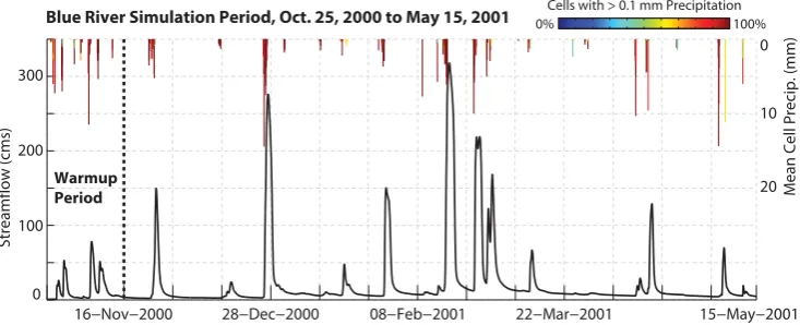
Fig. 1b, resulting in a total basin area of 1248 km2. The model was forced using hourly NEXRAD precipitation data over the 6 month period from 16 November 2000 to 15 May 2001, preceded by a 3 week warmup period. Figure 2 shows the hourly precipitation and streamflow data for the Blue River during the selected simulation period. As Fig. 2 indi-cates, the Blue River remains at low flow during much of the simulation period, punctuated by a series of large rainfall events.
3 Sensitivity analysis methods
3.1 Sobol0sensitivity analysis
Sobol0 sensitivity analysis (Sobol0, 2001; Saltelli, 2002) is a global, variance-based method that attributes variance in the model output to individual parameters and the interac-tions between parameters. In general, the attribution of to-tal output variance to individual model parameters and their interactions can be written as
D(f )=X
i
Di+ X i<j
Dij+ X i<j <k
Dij k+D12...p, (1)
whereD(f )represents the total variance of the output met-ricf;Di is the first-order variance contribution of thei-th
parameter,Dij is the second-order contribution of the
inter-action between parametersiandj; andD12...p contains all
interactions higher than third-order, up toptotal parameters.
The first-order and total-order sensitivity indices are defined as follows.
First-order index: Si =
Di
D (2)
Total-order index: STi =1−
D∼i
D (3)
The first-order index measures the fraction of the total output variance caused by the parameteri apart from interactions with other parameters. The total order index is one minus the fraction of total variance attributed toD∼i, which
repre-sents all parameters excepti. The total order index removes parameterifrom the analysis and attributes the resulting re-duction in variance to that parameter (Homma and Saltelli, 1996). The difference between a parameter’s first and total order indices represents the effects of its interactions with other parameters. In this study, we analyze the total order in-dices to determine the ranking of the most sensitive model parameters and compare these to the relatedµ∗statistic from the method of Morris.
Sobol0 sensitivity indices were calculated according to
the methods proposed by Sobol0and Saltelli (Sobol0, 2001;
[image:3.595.127.467.60.320.2]16−Nov−2000 28−Dec−2000 08−Feb−2001 22−Mar−2001 15−May−2001 0
10
100 200 300
Streamflow (cms)
0
20 Mean Cell Precip. (mm)
0%Cells with > 0.1 mm Precipitation100%
Warmup Period
[image:4.595.115.482.64.213.2]Blue River Simulation Period, Oct. 25, 2000 to May 15, 2001
Fig. 2. The hourly hydrograph of the 6 month simulation period for the Blue River basin, with a 3 week warm up period. The precipitation
amounts are based on the mean value across the 78 HRAP grid cells in the basin. The colors of the precipitation bars indicate the fraction of grid cells receiving more than 0.1 mm precipitation, representing the spatial distribution of each hourly rainfall value.
output values,f, which have a total varianceDas follows:
f0=
1 n
n X s=1
f (θs), (4)
D=1
n
n X s=1
f2(θs)−f02. (5)
Here, f0 is the mean of the distribution of model outputs
andθs represents the parameter set associated with sample
s. Equations (4) and (5) represent the mean and variance cal-culations proposed in Saltelli et al. (2008). For adaptations to these calculations, which aim to improve the convergence of Sobol0indices, the reader is referred to Saltelli (2002) and Nossent and Bauwens (2012b).
The variance contributionsDi andD∼i are calculated
ac-cording to Sobol0(2001) and Saltelli et al. (2008). First, two matrices A and B are each assignedN sampled parameter sets. The sample set A is used to calculate the total variance as shown in Eqs. (4) and (5). The sample set B is used to resample or fix each parameter as necessary in the following expressions:
Di=
1 n
n X s=1
f
θsA
f
θ∼isB , θisA
−f02, (6)
D∼i=
1 n
n X s=1
fθsAfθ∼isA , θisB−f02. (7)
In Eqs. (6) and (7), the parameter setsθi are superscripted
to indicate which parameters are sampled from which set. The sample set is denoted by the superscriptAorB; the pa-rameters taken from that set are denoted either byi(thei-th parameter) or∼i(all parameters excepti). This scheme al-lows the estimation of first and total order sensitivity indices with a total ofN (p+2)model evaluations, wherepis the number of parameters for which indices are to be calculated.
3.2 Method of Morris
The method of Morris (1991) derives measures of global sen-sitivity from a set of local derivatives, or elementary effects, sampled on a grid throughout the parameter space. It is based on one-at-a-time (OAT) methods, in which each parameter xi is perturbed along a grid of size 1i to create a
trajec-tory through the parameter space. For a given model with p parameters, one trajectory will contain a sequence of p such perturbations. Each trajectory yields one estimate of the elementary effect for each parameter (i.e., the ratio of the change in model output to the change in that parameter). Equation (8) shows the calculation of a single elementary effect for thei-th parameter.
EEi=
f (x1, . . . , xi+1i, . . . , xp)−f (x)
1i
(8) wheref (x)represents the prior point in the trajectory. In al-ternative formulations, both the numerator and denominator are normalized by the values of the function and parameter xi, respectively, at the prior point x (van Griensven et al.,
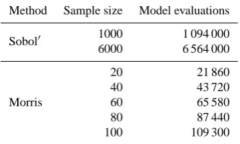
Table 1. Sample sizes and number of model runs performed for
each of the sensitivity analysis methods.
Method Sample size Model evaluations
Sobol0 1000 1 094 000
6000 6 564 000
Morris
20 21 860
40 43 720
60 65 580
80 87 440
100 109 300
suggest promising directions for future investigation. Once trajectories are sampled, the resulting set of elementary ef-fects is then averaged to giveµ, which serves as an estimate of total-order effects. Similarly, the standard deviation of the set of elementary effectsσdescribes the variability through-out the parameter space and thus the extent to which parame-ter inparame-teractions are present. This study uses the improvement of Campolongo et al. (2007) in which an estimate of total-order sensitivity of thei-th parameter,µ∗i, is computed from the mean of the absolute values of the elementary effects over the set ofN trajectories as shown in Eq. (9).
µ∗i = 1
N
N X j=1
EE
j i
(9)
4 Computational experiment
The sensitivity analyses were performed on the 14 SAC-SMA model parameters as indicated in Fig. 1. The lower and upper bounds for each parameter are based on the a pri-ori gridded parameter values derived by the NWS (Ko-ren et al., 2004) and extended for sensitivity analysis by Van Werkhoven et al. (2008b). These parameter ranges are included in the Supplement. Parameter values for each grid cell were sampled separately from uniform distributions. Rather than measure the sensitivity of the output stream-flow directly, we measure the sensitivity of the root mean squared error (RMSE) metric, calculated using the known hourly streamflow values over the 6 month simulation pe-riod. This ensures that our sensitivity indices are grounded relative to the observed streamflow and describe the controls on model performance.
The sample sizes and corresponding number of model evaluations required for both the Sobol0and Morris methods
are shown in Table 1. For the Sobol0 method, sample sizes ofN= 1000 andN= 6000 were used, resulting in just over 1 million and 6 million model evaluations, respectively. The latter value represents the limit of computational feasibility for this model at an hourly time step, to derive maximally ac-curate baseline values of the sensitivity indices. The two sam-ple sizes were employed to verify convergence of the Sobol0
indices. Confidence intervals for the sensitivity indices de-rived from the bootstrap method (Efron and Tibshirani, 1994; Archer et al., 1997) were monitored to ensure convergence of the Sobol0 method at the N= 6000 level. Convergence was considered acceptable if the 95 % confidence interval repre-sented less than 10 % of the sensitivity index value for the most sensitive parameters. For the method of Morris, sam-ple sizes ranging from N= 20 to N= 100 were chosen to determine if the approach can provide suitable results with orders of magnitude fewer model evaluations. Open-source implementations were used for the methods of Morris (Pu-jol et al., 2013) and Sobol0 sensitivity analysis (Hadka and Reed, 2012). The sensitivity analyses were performed us-ing the CyberSTAR high-performance cluster at Penn State University, which contains a combination quad-core AMD Shanghai processors (2.7 GHz) and Intel Nehalem processors (2.66 GHz). Approximately 50 000 computing hours were required to complete the experiment.
5 Results and discussion
The results of the sensitivity analyses can be addressed through the lens of two primary questions: (1) what is the sample size required for the Sobol0 method to return reli-able sensitivity indices; and (2) how suitreli-able are the indices returned by the method of Morris relative to the baseline created by the Sobol0method.
5.1 Convergence of Sobol0indices
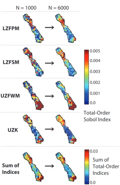
Figure 3 shows the spatial maps of total-order Sobol0
sensi-tivity indices for the sample sizesN= 1000 and N= 6000. The four most sensitive parameters of the SAC-SMA model are shown, as well as the cell-level sum of sensitivity in-dices. The total-order indices vary over a small range since the output variance must be distributed across the full set of distributed parameters, 1092 in total.
Figure 3 reveals several interesting spatial patterns of sen-sitivity. First, the most sensitive parameters are primarily up-per and lower storage zone maxima. The lower-zone storage maxima, LZFPM (lower-zone free primary maximum) and LZFSM (lower-zone free water supplemental maximum), are most sensitive in the headwater portion of the basin, while the upper-zone storage maximum UZFWM (upper-zone free water storage) is most sensitive toward the outlet of the basin. The resulting summation of sensitivity indices shows a division of the most active cells, with one group in the headwaters and another near the outlet.
LZFPM
LZFSM
0.0 0.001 0.002 0.003 0.004 0.005
UZFWM
UZK
Sum of Indices
0.0 0.03
N = 1000 N = 6000
Total-Order Sobol Index
[image:6.595.67.267.75.382.2]Sum of Total-Order Indices
Convergence of Sobol Indices
Fig. 3. Maps of the total-order Sobol0sensitivity indices for the four most sensitive parameters as well as the total sum in each grid cell.
The maps are shown for theN= 1000 andN= 6000 sample sizes.
The lower sample size shows a coarse identification of sensitive and
insensitive cells. TheN= 6000 sample size shows smoother spatial
patterns of sensitivity indices, suggesting that this level of sampling
is required for reliable Sobol0indices.
indices in Fig. 3 can be interpreted in the context of the sev-eral high-flow events shown in the hydrograph in Fig. 2. To-ward the outlet of the basin, the primary runoff-generating mechanisms in the model are overflow exceeding UZFWM and drainage from the upper zone (controlled by UZK, the upper-zone drainage coefficient). The fact that the lower-zone drainage constants LZPK (lower-lower-zone primary coeffi-cient) and LZSK (lower-zone secondary coefficoeffi-cient) are not sensitive indicates that they act on a slower timescale and thus do not affect RMSE. In the headwaters, the lower zone storage maxima (LZFPM and LZFSM) and the rate constant UZK are most sensitive, likely because these parameters must not allow too much direct runoff from the headwater region to prevent the model from overshooting the observed flow peaks and causing poor RMSE performance. While the temporal distribution of forcing can affect the sensitivity in-dices shown in Fig. 3, the spatial distribution can be restricted to the processes occurring within the model.
Also visible in Fig. 3 is the difference in Sobol0
sensitiv-ity indices as a function of sample size. At a sample size ofN= 1000, the most sensitive cells are identified, but it is clear that cells with intermediate sensitivity values largely remain unidentified. For example, it is common to see sen-sitive cells (red) adjacent to insensen-sitive cells. Intuitively, we should expect to see a smoother spatial gradient of sensitivity in which the most sensitive cells are adjacent to intermediate-sensitivity cells, which in turn are adjacent to low-intermediate-sensitivity cells. This is achieved to a larger extent with a sample size of N= 6000. Here, the sensitivity indices vary more smoothly in space, indicating that theN= 6000 case provides a base-line for total-order sensitivity indices. The bootstrap confi-dence intervals confirm convergence for theN= 6000 sam-ple size. TheN= 1000 case would not be sufficient to cap-ture the full range of sensitivity, a fact that underscores the high computational requirements of the Sobol0method. It is
worth noting that the slow convergence of the Sobol0method
for this model is related to the large number of parame-ters over which variance must be decomposed, leading to small sensitivity values and a correspondingly narrow range of acceptable confidence bounds (see Nossent et al., 2011).
5.2 Comparison of Sobol0and Morris indices
The Sobol0sensitivity indices from theN= 6000 case form a set of target values against which the method of Morris will be compared. Figure 4 compares this target to the lowest-sample Morris experiment, N= 20, for all 14 of the SAC-SMA parameters and the sums of parameter indices for each of the 78 grid cells. The Sobol0indices offer a quantitative
interpretation as a fraction of total variance, but the Morris indices do not; the latter are mapped from the range(0,0.1) to(0,1)to avoid this misinterpretation.
Figure 4 shows that the total-order indices calculated by the method of Morris with only N= 20 samples success-fully capture the spatial patterns of the Sobol0 indices with N= 6000 samples. The Morris indices are able to isolate the most sensitive parameters, along with their correct loca-tions in the watershed: LZFPM, LZFSM, and UZK in the headwaters, and UZFWM, UZK, and ADIMP (additional impervious area) near the outlet. It also correctly identifies the parameters that are insensitive over the simulation pe-riod: LZTWM (lower zone tension water maximum), PC-TIM (percent of impervious area), PFREE (percolation co-efficient), UZTWM (upper-zone tension water maximum), and RIVA (riparian vegetation area). The sums of indices are also comparable between the Sobol0and Morris methods,
LZFPM
LZFSM
LZPK
LZSK
LZTWM
PCTIM
PFREE
REXP
UZFWM
UZK
UZTWM
ZPERC
ADIMP
RIVA
Sums of Sobol and Morris Indices
Sobol N=6000
0.0
0.005 Total-Order Sobol Index
Morris N=20
0.0
1.0 Morris μ* Value (Scaled)
Comparison of Sobol (N = 6000) and Method of Morris (N = 20) Sensitivity Results
0.0
1.0 Sum of μ* Values (Scaled)
0.0
0.03 Sum of Total-Order Sobol Indices
HL-RDHM Parameters
Fig
.
4.
T
otal-order
sensiti
vity
indices
calculated
by
the
Sobol
0method,
with
sample
size
N
=
6000,
and
the
method
of
Morris,
with
N
=
20.
The
Morris
indices
are
normalized
to
the
range
(
0
,
1
)
since
the
y
do
not
of
fer
a
quantitati
v
e
interpreta
tion
of
percent
v
ariance.
The
method
of
Morris
is
able
to
correctly
identify
sensiti
v
e
and
insensiti
v
e
parameters,
as
we
ll
as
their
spatial
patterns,
with
far
fe
wer
model
ev
aluations.
The
sums
of
sensiti
vity
indices
represent
the
addition
of
parameter
indices
within
ea
ch
grid
0 0.01 0.02
Sobol Total−Order Index, N=6000
0 0.01 0.02 0 0.01 0.02 0 0.01 0.02 0 0.01 0.02
0 0.2 0.4 0.6 0.8 1.0
Morris
µ
* Value (Scaled)
1
500
1092
Morris Parameter Rank
1 500
1092 1092 500 1 1092 500 1 1092 500 1 1092 500 1
Sobol Parameter Rank, N=6000 N = 20
ρ = 0.885 N = 40ρ = 0.896 N = 60ρ = 0.897 N = 80ρ = 0.898 N = 100ρ = 0.898
N = 20 R2 = 0.89
N = 40 R2 = 0.90
N = 60 R2 = 0.90
N = 80 R2 = 0.91
[image:8.595.97.496.65.321.2]N = 100 R2 = 0.91 Comparison of Sensitivity Indices and Parameter Ranks
Fig. 5. Statistical comparison of sensitivity indices and sensitivity ranks (1–1092) between the Sobol0method (N= 6000) and the method of
Morris with sample sizes fromN= 20 toN= 100. The sensitivity indices are compared using a nonlinear Spearman correlation coefficient
(ρ), while the rankings are compared with a linear correlation coefficient (R2). Each plot contains all 14 parameters from each grid cell, for
a total of 1092 points.
102 103 104 105
0 60 120 180
Runtime (hours)
Storage (GB)
Time and Storage Requirements
Sobol
N = 1000 N = 6000
Method of Morris
N = 20 N = 100
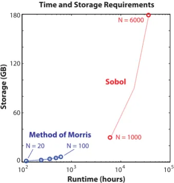
Fig. 6. Computation time (hours) and storage (gigabytes) required
for each experiment. The method of Morris with N= 20
repre-sents a factor of 300 computational savings compared to the Sobol0
method withN= 6000.
patterns, at greatly reduced computational expense relative to the Sobol0method.
The Morris sensitivity indices can also be compared sta-tistically to the Sobol0 indices for theN= 6000 case to en-sure sufficient similarity. Figure 5 compares the sensitivity
indices for each method, as well as the sensitivity ranks (1– 1092), for all of the Morris sample sizes from N= 20 to N= 100. The sensitivity indices are compared using a non-linear Spearman correlation coefficient, because a one-to-one correspondence between Sobol0 and Morris indices is not necessary. The rankings are compared with a linear corre-lation coefficient, because ideally these will exhibit a one-to-one correspondence.
The top panels in Fig. 5 show that the Morrisµ* values for all sample sizes are well-correlated with the Sobol0 indices with a sample size ofN= 6000. Importantly, there appears to be little benefit in running the method of Morris for sam-ple sizes greater thanN= 20, since the correlation remains similar for higher sample sizes. The relationship between Morrisµ* values and Sobol0indices is approximately linear for low-sensitivity parameters. However, the relationship be-comes nonlinear for high-sensitivity parameters, where the Morris µ* values appear to flatten out. This suggests that the method of Morris cannot reliably reproduce the precise ranking of high-sensitivity parameters provided by the Sobol0 method. However, the method of Morris successfully distin-guishes sensitive from insensitive parameters, and a sample size ofN= 20 is clearly sufficient to achieve this.
[image:8.595.82.252.399.578.2]a sample size ofN= 20 for the method of Morris appears suf-ficient to achieve a good correlation, and little is gained by in-creasing the sample size further. Of particular interest are the clusters of highly correlated parameters ranked near the most and least sensitive (ranks 1 and 1092, respectively). This in-dicates that the method of Morris can isolate the most and least sensitive parameters with high reliability, reinforcing its utility as a screening method. The outliers in the bottom pan-els in Fig. 5 reinforce the difficulty for the method of Mor-ris to distinguish between sensitive parameters; it correctly identifies them as sensitive, but struggles to rank them quan-titatively. The largest outliers occur in the upper-left of each plot, where the method of Morris attributes erroneously high rankings to certain parameters. These outliers correspond to parameters of average rank, whose low (but non-zero) sen-sitivity values are extremely difficult to differentiate from one another. Thus, these points highlight the limitations of the method of Morris for this model, but they do not detract from the success of the approach in correctly classifying the parameters with the highest and lowest sensitivity values.
Given that both the spatial and statistical comparisons be-tween the Sobol0and Morris sensitivity indices indicate the success of the method of Morris, it is worth exploring the amount of computation saved to achieve a highly similar set of sensitivity results. Figure 6 shows the location of each experiment in the space defined by the computation time and storage required. The largest Sobol0 experiment, with N= 6000, required over 6 million model evaluations, lead-ing to more than 30 000 h of computation time and approx-imately 180 gigabytes of storage space to store the model output. By contrast, the smallest Morris experiment, with N= 20, required roughly 100 h of computation and 1 giga-byte of storage space. This represents a factor of 300 sav-ings in both the runtime and storage dimensions relative to the Sobol0 method. As shown in Figs. 4 and 5, the sensitiv-ity indices calculated by this lowest-sample Morris experi-ment are spatially and statistically comparable to those cal-culated by the highest-sample Sobol0experiment. The Sobol0 method confers several advantages, including the first order sensitivity indices, and a large ensemble of model evalua-tions to be used in an uncertainty analysis or likelihood-based optimization framework, which the method of Morris does not provide. However, for the purpose of obtaining an ac-curate distinction between sensitive and insensitive param-eters, it is clear that the method of Morris provides signif-icant computational savings without signifsignif-icant degradation of solution quality.
6 Conclusions
The method of Morris is able to correctly screen the most and least sensitive parameters for a highly parameterized, spatially distributed watershed model with 300 times fewer model evaluations than the Sobol0 method. Even for this
complex model, the efficient factorial sampling scheme of the method of Morris is sufficient to isolate the controls on model performance without any prior assumptions on the form of the model output. For many distributed modeling ap-plications, the Sobol0 method requires a prohibitive number of model evaluations. In light of these results, the method of Morris proves to be a promising way forward for effi-cient global sensitivity analysis of distributed models. It also holds promise as a screening technique, identifying parame-ters that can safely be removed prior to more complex anal-yses such as the Sobol0method or model calibration. Future work will include an investigation of time-varying sensitiv-ity to determine the extent to which spatial sensitivsensitiv-ity pat-terns change during wet and dry periods. The increasing use of spatially distributed hydrologic models requires that diag-nostics such as these sensitivity analysis methods be evalu-ated not only in terms of their statistical effectiveness but also by their efficiency, to ensure that hydrologic modelers can obtain maximally reliable diagnostic insights at a reasonable computational cost.
Supplementary material related to this article is
available online at: http://www.hydrol-earth-syst-sci.net/ 17/2893/2013/hess-17-2893-2013-supplement.pdf.
Acknowledgements. The authors of this work were partially sup-ported by the US National Science Foundation under grant EAR-0838357. The computational resources for this work were provided in part through instrumentation funded by the National Science Foundation through grant OCI-0821527. Any opinions, findings, and conclusions are those of the authors and do not necessarily re-flect the views of the US National Science Foundation.
Edited by: F. Pappenberger
References
Alton, P., Mercado, L., and North, P.: A sensitivity analysis of the land-surface scheme JULES conducted for three forest biomes: Biophysical parameters, model processes, and meteo-rological driving data, Global Biogeochemical Cy., 20, GB1008, doi:10.1029/2005GB002653, 2006.
Archer, G., Saltelli, A., and Sobol, I.: Sensitivity measures, ANOVA-like techniques and the use of bootstrap, J. Stat. Com-put. Simul., 58, 99–120, 1997.
Bastidas, L., Hogue, T., Sorooshian, S., Gupta, H., and Shuttle-worth, W.: Parameter sensitivity analysis for different complex-ity land surface models using multicriteria methods, J. Geophys. Res., 111, 20101, doi:10.1029/2005JD006377, 2006.
Campolongo, F., Cariboni, J., and Saltelli, A.: An effective screen-ing design for sensitivity analysis of large models, Environ. Mod-ell. Softw., 22, 1509–1518, 2007.
Campolongo, F., Saltelli, A., and Cariboni, J.: From screening to quantitative sensitivity analysis. A unified approach, Comput. Phys. Commun., 182, 978–988, 2011.
Carpenter, T. M., Georgakakos, K. P., and Sperfslagea, J. A.: On the parametric and NEXRAD-radar sensitivities of a distributed hydrologic model suitable for operational use, J. Hydrol., 253, 169–193, 2001.
Cloke, H., Pappenberger, F., and Renaud, J.: Multi–method global sensitivity analysis (MMGSA) for modelling floodplain hydro-logical processes, Hydrol. Process., 22, 1660–1674, 2008. Demaria, E., Nijssen, B., and Wagener, T.: Monte Carlo
sensi-tivity analysis of land surface parameters using the Variable Infiltration Capacity model, J. Geophys. Res, 112, D11113, doi:10.1029/2006JD007534, 2007.
Efron, B. and Tibshirani, R. J.: An introduction to the bootstrap, Vol. 57, Chapman & Hall/CRC, 1994.
Franchini, M., Wendling, J., Obled, C., and Todini, E.: Physical in-terpretation and sensitivity analysis of the TOPMODEL, J. Hy-drol., 175, 293–338, 1996.
Freer, J., Beven, K., and Ambroise, B.: Bayesian estimation of un-certainty in runoff prediction and the value of data: An applica-tion of the GLUE approach, Water Resour. Res., 32, 2161–2173, 1996.
Gupta, Wagener, T., and Liu, Y.: Reconciling theory with obser-vations: elements of a diagnostic approach to model evaluation, Hydrolog. Process., 22, 3802–3813, 2008.
Gupta, H., Sorooshian, S., and Yapo, P.: Toward improved cali-bration of hydrologic models: Multiple and noncommensurable measures of information, Water Resour. Res., 34, 751–763, 1998. Hadka, D. and Reed, P.: MOEAFramework: An open-source Java framework for multiobjective optimization, available at: http:// moeaframework.org, version 1.17, 2012.
Hall, J., Tarantola, S., Bates, P., and Horritt, M.: Distributed sensi-tivity analysis of flood inundation model calibration, J. Hydraul. Eng., 131, 117–126, 2005.
Herman, J. D., Reed, P. M., and Wagener, T.: Time-varying sen-sitivity analysis clarifies the effects of watershed model formu-lation on model behavior, Water Resour. Res., 49, 1400–1414, doi:10.1002/wrcr.20124, 2013.
Homma, T. and Saltelli, A.: Importance measures in global sensi-tivity analysis of nonlinear models, Reliability Eng. Syst. Safe., 52, 1–17, 1996.
Hornberger, G. and Spear, R.: Approach to the preliminary analysis of environmental systems, J. Environ. Manage., 12, 7–18, 1981. Koren, V., Reed, S., Smith, M., Zhang, Z., and Seo, D.-J.:
Hydrol-ogy laboratory research modeling system (HL-RMS) of the US national weather service, J. Hydrol., 291, 297–318, 2004. Moreda, F., Koren, V., Zhang, Z., Reed, S., and Smith, M.:
Pa-rameterization of distributed hydrological models: learning from the experiences of lumped modeling, J. Hydrol., 320, 218–237, 2006.
Morris, M. D.: Factorial Sampling Plans for Preliminary Com-putational Experiments, Technometrics, 33, 161–174, Article-Type: research-article/Full publication date: May, 1991/Copy-right1991 American Statistical Association and American Soci-ety for Quality, 1991.
Muleta, M. and Nicklow, J.: Sensitivity and uncertainty analysis coupled with automatic calibration for a distributed watershed model, J. Hydrol., 306, 127–145, 2005.
Nossent, J. and Bauwens, W.: Application of a normalized Nash-Sutcliffe efficiency to improve the accuracy of the Sobol’sensitivity analysis of a hydrological model, in: EGU General Assembly Conference Abstracts, 14, p. 237, avail-able at: http://adsabs.harvard.edu/abs/2012EGUGA..14..237N, 2012a.
Nossent, J. and Bauwens, W.: Optimising the convergence of Sobol sensitivity analysis for an environmental model: application of an appropriate estimate for the square of the expectation value and total variance, in: International Environmental Modelling and Software Society 2012 International Congress on Environmen-tal Modelling and Software. Managing Resources of a Limited Planet: Pathways and Visions under Uncertainty, Sixth Biennial Meeting, Leipzig, Germany, edited by: Seppelt, R., Voinov, A., Lange, S., and Bankamp, D., 1080–1087, 2012b.
Nossent, J., Elsen, P., and Bauwens, W.: Sobol sensitivity analysis of a complex environmental model, Environ. Modell. Softw., 26, 1515–1525, 2011.
Pujol, G., Iooss, B., and Janon, A.: Sensitivity Analysis Package, available at: http://cran.r-project.org/web/packages/sensitivity/ index.html, R package version 1.7-0, 2013.
Reed, S., Koren, V., Smith, M., Zhang, Z., Moreda, F., Seo, D.-J., and DMIP Participants, A.: Overall distributed model intercom-parison project results, J. Hydrol., 298, 27–60, 2004.
Reusser, D. and Zehe, E.: Inferring model structural deficits by analyzing temporal dynamics of model performance and parameter sensitivity, Water Resour. Res., 47, W07550, doi:10.1029/2010WR009946, 2011.
Reusser, D., Buytaert, W., and Zehe, E.: Temporal dynamics of model parameter sensitivity for computationally expensive mod-els with the Fourier amplitude sensitivity test, Water Resour. Res., 47, W07551, doi:10.1029/2010WR009947, 2011. Ruano, M., Ribes, J., Seco, A., and Ferrer, J.: An improved
sam-pling strategy based on trajectory design for application of the Morris method to systems with many input factors, Environ. Modell. Softw., 37, 103–109, 2012.
Saltelli, A.: Making best use of model evaluations to compute sen-sitivity indices, Comput. Phys. Commun., 145, 280–297, 2002. Saltelli, A., Ratto, M., Andres, T., Campolongo, F., Cariboni, J.,
Gatelli, D., Saisana, M., and Tarantola, S.: Global sensitivity analysis: the primer, Wiley Online Library, 2008.
Sieber, A. and Uhlenbrook, S.: Sensitivity analyses of a distributed catchment model to verify the model structure, J. Hydrol., 310, 216–235, 2005.
Smith, M. B., Seo, D.-J., Koren, V. I., Reed, S. M., Zhang, Z., Duan, Q., Moreda, F., and Cong, S.: The distributed model intercompar-ison project (DMIP): motivation and experiment design, J. Hy-drol., 298, 4–26, 2004.
Smith, M. B., Koren, V., Reed, S., Zhang, Z., Zhang, Y., Moreda, F., Cui, Z., Mizukami, N., Anderson, E. A., and Cosgrove, B. A.: The distributed model intercomparison project – Phase 2: Moti-vation and design of the Oklahoma experiments, J. Hydrol., 418– 419, 3–16, 2012.
Sobol0, I.: Global sensitivity indices for nonlinear mathematical
Tang, Y., Reed, P., Van Werkhoven, K., and Wagener, T.: Advanc-ing the identification and evaluation of distributed rainfall–runoff models using global sensitivity analysis, Water Resour. Res., 43, W06415, doi:10.1029/2006WR005813, 2007a.
Tang, Y., Reed, P., Wagener, T., and van Werkhoven, K.: Comparing sensitivity analysis methods to advance lumped watershed model identification and evaluation, Hydrol. Earth Syst. Sci., 11, 793– 817, doi:10.5194/hess-11-793-2007, 2007b.
van Griensven, A., Meixner, T., Grunwald, S., Bishop, T., Diluzio, M., and Srinivasan, R.: A global sensitivity analysis tool for the parameters of multi-variable catchment models, J. Hydrol., 324, 10–23, 2006.
Van Werkhoven, K., Wagener, T., Reed, P., and Tang, Y.: Characterization of watershed model behavior across a hy-droclimatic gradient, Water Resour. Res., 44, W01429, doi:10.1029/2007WR006271, 2008a.
Van Werkhoven, K., Wagener, T., Reed, P., and Tang, Y.: Rainfall characteristics define the value of streamflow observations for distributed watershed model identification, Geophys. Res. Lett, 35, L11403, doi:10.1029/2008GL034162, 2008b.
Van Werkhoven, K., Wagener, T., Reed, P., and Tang, Y.: Sensitivity–guided reduction of parametric dimensionality for multi–objective calibration of watershed models, Adv. Water Re-sour., 32, 1154–1169, 2009.
Wagener, T., Boyle, D. P., Lees, M. J., Wheater, H. S., Gupta, H. V., and Sorooshian, S.: A framework for development and applica-tion of hydrological models, Hydrol. Earth Syst. Sci., 5, 13–26, doi:10.5194/hess-5-13-2001, 2001.
Wagener, T., Reed, P., van Werkhoven, K., Tang, Y., and Zhang, Z.: Advances in the identification and evaluation of complex envi-ronmental systems models, J. Hydroinform., 11, 266–281, 2009. Yang, J.: Convergence and uncertainty analyses in Monte–Carlo based sensitivity analysis, Environ. Modell. Softw., 26, 444–457, 2011.