Discretization based Support Vector Machine
(D-SVM) for Classification of Agricultural Datasets
Anshu Bharadwaj Shashi Dahiya Rajni Jain
IASRI, Library Avenue, IASRI, Library Avenue NCAP, Library Avenue New Delhi-110012 New Delhi-110012 New Delhi-110012
ABSTRACT
Discrete values have important roles in data mining and knowledge discovery. They are about intervals of numbers which are concise to represent and specify, easier to use and comprehend as they are closer to the knowledge level representation than continuous ones. Data is reduced and simplified using discretization and it makes the learning more accurate and faster [3]. Support Vector Machine (SVM) developed by [15] is a novel learning method based on statistical learning theory. SVM is a powerful tool for solving classification problems with small samples, nonlinearities and local minima, and has been of excellent performance. In this paper, a new approach to classify data using discretization based SVM classifier, is discussed. This is an attempt to extend the boundaries of discretization and to evaluate its effect on other machine learning techniques for classification namely, support vector machines.
General Terms:
Classification, Support Vector Machine, DiscretizationKeywords:
Classification, Data-preprocessing, Discretization, Support Vector Machine, Confusion MAtrix1.
INTRODUCTION
Support Vector Machine (SVM) is a novel learning method based on statistical learning theory. SVM is a powerful tool for solving classification problems with small samples, nonlinearities and local minima, and is of excellent performance. To address the discretization process of continuous-valued features in an efficient and proper manner has always been an important issue for any machine learning technique. Support vector machine is a widely used method for classification and have been used in variety of applications. The results of the experiment conducted in this study clearly show that the classification results using SVM are better when discretization of data is undertaken before the classification. However, various methods of discretization affect the classification accuracy. Therefore, it is important to decide a method to improve the performance of the SVM model. The points in the dataset that fall on the bounding planes of the hyperplane in a support vector machines are called support vectors. They play an important role in the theory as well as in the classification task at the prediction stage. Vapnik [13,14,15] has shown that if the training vectors are separated without errors by an optimal hyperplane, the expected error rate on a test sample is bounded by the ratio of the expectation of the support vectors to the number of training vectors. Since this ratio is independent of the dimension of the problem, and, if good set of support vectors can be found, good generalization is guaranteed. A good generalization is the objective from the classification task that
is carried out using SVM after discretization. Even though support vector machines can handle continuous attributes, its performance can be significantly improved by replacing a continuous attribute with its discretized values. Data discretization is defined as a process of converting continuous data attribute values into a finite set of intervals and associating with each interval some specific data value. There are no restrictions on discrete values associated with a given data interval except that these values must induce some ordering on the discretized attribute domain. Discretization significantly improves the quality of discovered knowledge [3], [10] and also reduces the running time of various data mining tasks such as association rule discovery, classification, and prediction. In this study, we have also used two spatial datasets. These datasets have been used to examine the performance of the classification technique used for classical data mining task on it. Spatial datasets differ from non-spatial datasets as they have spatial aspects involved in it. Here, the spatial datasets used are in the vector format. The spatial attributes in the spatial datasets used, are latitudes and longitudes. The datasets were considered just to experiment with it using discretization based SVM classifier. In this paper, we have used Entropy method of discretization. We focus our work to find out the significance of discretization before classification using SVM.
This paper is organized as follows: Section 2 gives the preliminaries about data pre-processing, discretization and Support Vector Machine. Section 3 describes the performance evaluation measure- Confusion Matrix. Section 4 gives the details of the Discretization based Support Vector Machine (D-SVM) model. Section 5 describes about the experimental setup, description of the data used and its analysis. Section 6 contains the results and section 7 draws conclusions.
2.
PRELIMINARIES
2.1 Data Pre-processing
grouping of values of symbolic attributes; Attribute selection and ordering; attribute construction and transformation; consistency checking. In this paper the data has been discretized as the pre-processing step before classification using SVM.
2.2 Discretization
Discretization of numerical attributes is one of the important data pre-processing techniques. Data discretization is defined as one of the way to reduce data used to change the original continuous attributes to discrete attributes [7]. It creates an appropriate number of intervals for data values thus transforming the continuous data values into the discrete values. The smaller data intervals usually contributed to more accurate predictive model which could cover higher prediction rates into new cases. Discretization is required particularly for rule-based data mining model such as decision tree and rough set classifiers [9]. In this paper, the datasets are discretized as the pre-processing step before classifying the data using SVM.
There are many advantages of using discrete values over continuous one. Discrete features are closer to knowledge level representation [11] than continuous ones. Data is reduced and simplified using discretization. For both users and experts, discrete features are easier to understand, use and explain. As reported in a study [5], discretization makes learning more accurate and faster. In general, obtained results using discrete features are usually more compact, shorter and more accurate than using continuous ones; hence the results can be more closely examined, compared, used and reused. In addition to the many advantages of having discrete data over continuous one, a suite of classification learning algorithms can only deal with discrete data.
2.3 Support Vector Machines (SVM)
The foundations of Support Vector Machines (SVMs) based on statistical learning theory have been developed by Vapnik [15] and Burges [2] to solve the classification problem. The support vector machine (SVM) is the recent addition to the toolbox of data mining practitioners and are gaining popularity due to many attractive features, and promising empirical performance. They are a new generation learning system based on the latest advances in statistical learning theory. The formulation embodies the Structural Risk Minimization (SRM) principle, which has been shown to be superior [6], to traditional Empirical Risk Minimization (ERM) principle, employed by conventional neural networks. SRM minimizes an upper bound on the expected risk, as opposed to ERM that minimizes the error on the training data. It is this difference which equips SVM with a greater ability to generalize, which is the goal in statistical learning. SVM belongs to the class of supervised learning algorithms in which the learning machine is given a set of examples (or inputs) with the associated labels (or output values). Like in decision trees, the examples are in the form of attribute vectors, so that the input space is a subset of Rn. SVMs create a hyperplane that separates two classes (this can be extended to multi class problems). While doing so, SVM algorithm tries to achieve maximum separation between the classes. Separating the classes with a large margin minimizes a bound on the expected generalization error. By “minimum generalization error”, it means that when new examples (data points with unknown class values) arrive for classification, the chance of making error in the prediction (of the class to which it belongs) based on the learned classifier (hyperplane) should be minimum. Intuitively, such a classifier is one which achieves maximum separation-margin between the classes.
The two planes parallel to the plane are called bounding planes. The distance between these bounding planes is called margin and by SVM “learning”, i.e. finding hyperplane which maximizes this margin. The points (in the dataset) falling on the bounding planes are called the support vectors. “Machine” in Support Vector Machines is nothing but the algorithm [12]. SVM was designed initially as binary classifier i.e. it classifies the data into two classes but researchers have extended its boundaries to be a multi-class classifier. SVM was first introduced as a training algorithm [1] that automatically tunes the capacity of the classification function maximizing the margin between the training patterns and the decision boundary [4]. This algorithm operates with large class of decision functions that are linear in their parameters but not restricted to linear dependences in the input components. For the computational considerations, SVM works well on the two important practical considerations of classification algorithms i.e. speed and convergence.
2.3.1 SVM and its parameter
To construct an optimal hyperplane, SVM employees an iterative training algorithm, this is used to minimize an error function. According to the form of the error function, SVM models can be classified into two distinct groups:
1. SVM for classification 2. SVM for regression
In this study we are dealing with classification problem, so the SVM for classification is described here. For SVM, training involves the minimization of the error function:
Ni i T
C
w
w
1
2
1
subject to the constraints:
i
iT
i
w
x
b
y
1
and
i
0
, i=1, …, Nwhere, C is the capacity constant or the model complexity, w
is the vector of coefficients, b a constant and iare
parameters for handling non-separable data (inputs). The
index i labels the N training cases. Note that
y
1
is the class label and xi is the independent variable. The kernel
is used to transform data from the input (independent) to the feature space. It should be noted that larger the C, the more the error is penalized. Thus, C should be chosen with care to avoid over fitting.2.3.2 Radial Basis Function (RBF)
There are a number of kernels that can be used for support vector machine models. These include Linear, Polynomial, Radial Basis and Sigmoid. A radial basis function (RBF) is a real-valued function whose value depends only on the distance
from the origin, so that ; or alternatively on the distance from some other point c, called a center, so
that . Any function that
are also possible. The following expression describes the RBF kernel for SVM:
2
exp
x
c
, where
>0
is called the RBF kernel parameter. The RBF kernel is themost popular kernel type due to its localized and finite response across the entire range of real x-axis.
3.
PERFORMANCE
EVALUATION
MEASURE: CONFUSION MATRIX
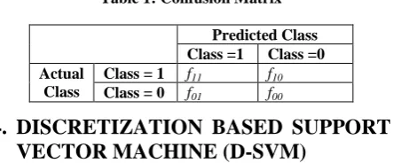
Evaluation of the performance of the classification model is based on the counts of the test records correctly or incorrectly predicted by the model. These counts are tabulated in a table called Confusion Matrix. Table 1 depicts the confusion matrix for a binary classification model. Each entry fij in this tabledenotes the number of records from class i predicted to be of class j. For instance f01 is the number of records from class 0
incorrectly predicted as of class 1. Based on the entries in the table the total number of correct prediction made by the model is (f11+ f00) and the total number of incorrect predictions is (f10
[image:3.595.59.281.344.436.2]+ f01).
Table 1: Confusion Matrix
Predicted Class Class =1 Class =0 Actual
Class
Class = 1 f11 f10
Class = 0 f01 f00
4.
DISCRETIZATION BASED SUPPORT
VECTOR MACHINE (D-SVM)
The proposed model works in two steps. The first step is the data pre-processing step in which the data is discretized and in the second step linear SVM is applied on the datasets for classification. The parameter selection or the parameter search of SVM decision function „C‟ i.e. capacity or model complexity, doesn‟t get affected by discretization as discretization process works on the
dataset rather than the model. Similarly, the parameter of the RBF kernel i.e. γ also remains unaffected by the discretization of the datasets before applying SVM.
For evaluation k-fold cross validation is used: first, the training set is split into k equal parts (called folds). Then, k training runs are performed, where each time, one part is left out and is used as an independent validation set. An individual's fitness is then the average of k validations. In k-fold cross validation, every data point appears once in the testing set, and k-1 times in the training set, thus reducing the dependence on how the data is divided. As k increases, the average performance estimate will be very accurate. However, computational time increases since the training algorithm is performed k - 1 times. The value of k used in this study is 10.
5.
EXPERIMENTS AND ANALYSIS
Using the discretization methods before applying SVM, it has been observed that discretization simplifies data (continuous values are quantized into intervals) without sacrificing data consistency much (only a few inconsistencies occur after discretization). The ultimate objective of discretization of the datasets, i.e.—whether discretization helps improve the performance of learning and understanding of learning results before applying SVM, has been evaluated The kernel used for
training is Radial Basis Function (RBF). The improvement is measured in terms of the classification accuracy. The evaluation of the performance of the classification model is done using Confusion Matrix. As a general approach of solving classification problems, each dataset is split into two datasets training sample dataset and test sample dataset. Training dataset consists of the records having class labels and is used to build the classification model whereas the test dataset contains records without class labels and is used to validate the model, built by training dataset. Though discretization is usually a needless pre-process step for SVM, which can deal with continuous and hybrid attributes directly, it has been still attractive to use discretized datasets because it has improved the classification performance and reduced the training time.
5.1 Data Description
Three agricultural datasets have been selected from different areas of Indian agriculture targeting different objectives to be carried out using classification task. The datasets selected and collected are from various sources and methods. The datasets are of varying sizes and have varying features. The first dataset is CIMMYT dataset. CIMMYT dataset is a live dataset. The live dataset used for this comparative study is Rice dataset. This dataset is in vector data format of spatial databases. Spatial attributes in the datasets are latitudes and longitudes. The data is obtained from Resource Conservation Technologies from Rice-Wheat Consortium, CIMMYT, India. Here, only a small part of data with 50 observations has been used for illustration purpose. There are 4 classes in which the data has to be classified. Number of attributes in the dataset is 10 including the class variable as well as the latitudes and longitudes being spatial attributes of the dataset. All the predictors are numeric. The CIMMYT dataset is modified as two different datasets: first by considering all the variables (latitudes and longitudes) as CIMMYT1, and secondly by ignoring the spatial variables, i.e. dropping the variables containing the spatial information, as CIMMYT2. The results may be different and the conclusions drawn here may change with the full set of data. The sample dataset is from different districts of Western Uttar Pradesh, India and contains different treatments (i.e. different kinds of seed cultivation), the spatial aspect of the location (longitudes and latitudes) with various biometrical characters of the rice plant. The task is to classify the varieties in different classes.
Second dataset is the Haryana Farmer data set. For performing classification task, dataset pertaining to the farmers from the State of Haryana in India is extracted from the 54th round dataset from National Sample Survey Organisation of India. The data is extracted for the reason that characteristics of technology savvy farmers are expected to be different for each state because of the geographical conditions also. The dataset contains 40 attributes including the decision attribute. The dataset contains 36 nominal as well as 4 real valued attributes. Haryana Farmers dataset contains 1832 cases. Aim of classification is to classify the farmers who will and who will not adopt pesticides.
their capability in taking decisions. The dataset contains 11 variables including a class variable. The predictors in the dataset are numeric as well as binary variable.
5.2 Experimental Setup and Analysis
D-SVM was run on 3 datasets. All the three datasets are real datasets collected from agriculture domain. They have been collected from two different states of India namely, Uttar Pradesh and Haryana. For comparing the D-SVM performance with SVM, the datasets were classified using SVM also.
The discretization of the datasets has been done in Rossetta software and SVM classification has been carried out in STATISTICA Data Miner of STATSOFT. Datasets have been discretized using supervised discretization algorithms namely Entropy method and Boolean Reasoning method and then the SVM classifier is applied. The kernel used for training the SVM is Radial Basis Function (RBF). SVM parameters have been tuned based on grid search method to find the best value of „C‟ and Gamma so as to improve classification. The improvement is measured in terms of the classification accuracy. The error rates have been estimated using 10x10 cross validation for all the datasets in the experiments conducted for this study. The evaluation of the performance of the classification model is done using Confusion Matrix. As a general approach of solving classification problems, each dataset is split into two datasets training dataset and test dataset. Training dataset consists of the records having class labels and is used to build the classification model whereas the test dataset contains records without class labels and is used to validate the model, built by training dataset. The splits used for the datasets are 70% to the training set and 30% to the testing set. The Discretization based SVM model has been used on both non-spatial and spatial datasets. The experiments were carried out and for each dataset; the results from a number of runs were obtained and averaged. For spatial datasets, an average of 10 runs is considered whereas for non-spatial datasets, an average of 05 runs has been averaged. The ultimate objective of discretization of the datasets before applying SVM—whether discretization helps improve the performance of learning and understanding of learning results has been evaluated. The results obtained have been studied to establish the usefulness of discretization before applying SVM with respect to the classification accuracy and also the effect of discretization based SVM model on classification of spatial datasets.
The datasets are split into train and test datasets, then the discretization algorithms (entropy based, boolean reasoning and equal-frequency) are used to discretize the train dataset one by one. Once the train dataset is discretized using any of the algorithms, the same cuts points [8] or intervals generated for the train dataset using the particular discretization algorithm are saved in a file and the same cuts points are then used to discretize the test dataset, for test dataset the class labels are not used during discretization. Once the data has been split (into train and test datasets) and discretized, the original dataset (i.e. the undiscretized data) has not been used anywhere in the study. The experiment was conducted with 8 runs each for each datasets. Each run, means to classify the data at split of different seed value. Seed values used for splits are 1000, 900, 800, 750, 600, 500, 350, 100. The seed values were randomly selected. Classification using SVM was carried out on the discretized datasets so that the results can be compared and the effect of the discretization on SVM can be
studied. CIMMYT dataset is spatial datasets in vector format with latitude and longitude as spatial attributes.
6.
RESULTS
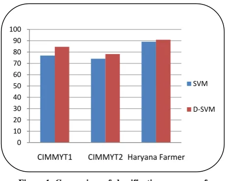
The results are shown in Table 2. Each result consists of the classification accuracy of the SVM learning technique with and without discretization of the datasets. On comparing the results of the algorithms, it was inferred that Discretization based Support Vector Machine (D-SVM) produced the model with highest accuracy for all the datasets (Table 2).
Table 2: Comparison of average accuracy of two classifiers
SVM classification using discretization (Fig. 1) shows that the results obtained are improved and better classification accuracy is attained. The parameter of SVM decision function i.e. capacity or model complexity doesn‟t get affected by discretization as discretization process works on the dataset rather than the model. Similarly, the parameter of the RBF kernel i.e. γ also remain unaffected by the discretization of the datasets before applying SVM.
[image:4.595.313.544.370.554.2]
Figure 1: Comparison of classification accuracy of D-SVM with SVM
Discretization yields the reduction in unique tuples by assigning the discretized value of the attribute to the objects whose numeric value lies in the corresponding discrete interval. Thus, we could observe that there had been a reduction in the number of support vectors per class during classification of the discretized dataset.
7.
CONCLUSION
The study was undertaken with an aim to explore the effects of discretization on support vector machines. Although data discretization has been a step for applying machine learning technique of classification such as decision tree but it has not been tried for support vector machines classifier, the reason being its ability to handle continuous and hybrid data unlike the decision tree algorithm ID3, which can handle only discrete datasets for classification. Therefore, it has been tried to explore the effect of discretization of the datasets before applying SVM classifier. This was done with the aim of
0 10 20 30 40 50 60 70 80 90 100
CIMMYT1 CIMMYT2 Haryana Farmer
SVM
D-SVM Technique CIMMYT1 CIMMYT2 Haryana
Farmer
SVM 76.85 74.00 89.10
attaining better classification accuracy without disturbing or distorting the parameters (C and γ) of SVM. The results clearly indicate that the accuracies of discretization based SVM are better as compared to the classification accuracy without SVM of the same datasets when they were classified without getting discretized.
8.
ACKNOWLEDGEMENTS
Authors are thankful to CIMMYT, India, for providing the data for carrying out this experiment.
9.
REFERENCES
[1] Boser, B.E, Guyon I.M, and Vapnik. V.N.1992. A Training Algorithm for Optimal Margin classifiers. In Proceedings of the 5th Annual Workshop on Computer Learning Theory, Pittsburgh, PA: ACM. pp. 144-152.
[2] Burges. J.C. 1998. A Tutorial on Support Vector Machines for Pattern Recognition. Data Mining and Knowledge Discovery. Vol. 2, pp121-167,
[3] Catlett. J.J. 1991. On Changing Continuous Attributes into Ordered Discrete Attributes. In the Proceedings of the Fifth European Working Session on Learning. Berlin: Springer-Verlag. pp.164-177.
[4] Cristianini N. and Shaw-Taylor. J. 2000. An Introduction to Support Vector Machines and Other Kernel-Based Learning Methods. Cambridge University Press,
Cambridge.
[5] Dougherty, J. Kohavi, R. and Sahami. M. 1995. Supervised and Unsupervised Discretization of Continuous Features. In Proceedings of the Twelfth International Conference on Machine Learning. Los Altos, CA: Morgan Kaufmann. pp 194-202.
[6] Gunn, S.R., M. Brown, and K.M. Bosely, 1997. Network Performance Assessment for Neurofuzzy Data Modelling . Intelligent Data Analysis, Vol. 1208, Lecture Notes in
Computer Science (X. Liu, P. Cohen, and M. Berthold (Eds.). pp. 313-323.
[7] Kraft, M.R., Desouza, K. C and Androwich, I. 2003. Data Mining in Healthcare Information Systems: Case Study of a Veterans' Administration Spinal Cord Injury Population. In the Proceedings of the 36th Annual Hawaii international Conference on System Sciences (Hicss'03). IEEE Computer Society, Washington. 6 (6): 159.1.
[8] Liu, Huan. Hussain, Farhad. Lan, Chew Tim and Dash,Manoranjan. (2002), Discretization: an enabling technique, Data Mining and Knowledge Discovery 6, pp.393-423.
[9] Mohd Shuib, N. L., Abu Bakar, A. and Othman, Z. A. 2009. In the Proceedings of the International Symposium on Computing, Communication, and Control (ISCCC 2009). Vol.1. (2011), pp. 305-308. IACSIT Press, Singapore.
[10] Pfahringer, B. 1995. Compression based discretization of continuous attributes. In the Proceedings of the Twelfth International Conference on Machine Learning. A. Prieditis & S. Russell, eds. Morgann Kauffman.
[11] Simon. H.A. 1981. The Sciences of the Artificial. 2nd Edn, Cambridge. MA. MIT.
[12] Soman, K.P. Diwakar, S. and Ajay. V. 2006. Insight into Data Mining: Theory and Practice. Prentice Hall of India Pvt. Ltd.
[13] Vapnik. V. 1974. Theory of Pattern Recognition. Nauka, Moscow.
[14] Vapnik V.and Chervonenkis. A. 1979. Theory of Pattern Recognition. Nauka, Moscow.