Implementation of Digital Video Broadcasting-Terrestrial
(DVB-T) using Orthogonal Frequency Division
Multiplexing (OFDM) on Physical Media Dependent
Sub layer
Sudipta Ghosh
Student, SECE Lovely Professional UniversityJalandhar, INDIA
Ankit Bass
Student, SECE Lovely Professional UniversityJalandhar, INDIA
ABSTRACT
Orthogonal frequency division multiplexing (OFDM) is a special case of multicarrier transmission, where a single data stream is transmitted over a number of lower rate subcarriers. Orthogonal frequency division multiplexing (OFDM) has been chosen as modulation technique for different application wireless communications. OFDM can provide large data rates with sufficient robustness to radio channel impairments. The purpose of this paper is to provide a MATLAB simulation of the basic processing involved in the generation and reception of an OFDM signal in a physical channel and to provide a description of each of the steps involved. For this purpose, we shall use one of the proposed OFDM signals of the Digital Video Broadcasting (DVB) standard for the European digital television service i.e. Digital Video Broadcast-Terrestrial (DVB-T).
General Terms
Fast fourier transform (FFT), Inverse fourier Transform (IFFT), Pulse Shaping, Filters
.
Keywords
Orthogonal Frequency Division Multiplexing (OFDM), Digital Video Broadcasting-Terrestrial (DVB-T)
1.
INTRODUCTION
Orthogonal frequency-division multiplexing (OFDM) is the modulation technique for European standards applications such as the Digital Audio Broadcasting (DAB) and the Digital Video Broadcasting (DVB) systems. As such it has received much attention and has been proposed for many other applications, including local area networks and personal communication systems. OFDM is a type of multichannel modulation that divides a given channel into many parallel subchannels or subcarriers, so that multiple symbols are sent in parallel. Earlier overviews of OFDM can be found in. The type of OFDM that we will describe in this article uses the discrete Fourier transform (DFT) with acyclic prefix. DFT (implemented with a fast Fourier transform (FFT)) and the cyclic prefix have made OFDM both practical and attractive to the radio link designer. A similar multichannel modulation scheme, discrete multitone (DMT) modulation, has been developed for static channels such as the digital subscriber loop. DMT also uses DFTs and the cyclic prefix but has the additional feature of bit-loading
which is generally not used in OFDM.
OFDM also has some drawbacks. Because OFDM divides a given spectral allotment into many narrow subcarriers each with inherently small carrier spacing, it is sensitive to carrier frequency errors. Furthermore, to preserve the orthogonality between subcarriers, the amplifiers need to be linear. OFDM systems also have a high peak-to-average power ratio or crest-factor, which may require a large amplifier power back-off and a large number of bits in the analog-to-digital (A/D) and digital-to-analog (D/A) designs. All these requirements can put a high demand on the transmitter and receiver design.
2.
ORTHOGONAL FREQUENCY
DIVISION MULTIPLEXING (OFDM)
OFDM is a multi-carrier modulation technique where data symbols modulate a sub-carrier which is taken from orthogonally separated sub-carriers with a separation of „fk‟ within each sub-carrier. Here, the spectra of sub-carrier are overlapping; but the sub-carrier signals are mutually orthogonal, which is utilizing the bandwidth very efficiently. To maintain the orthogonality, the minimum separation between the sub-carriers should be „fK‟ to avoid ICI (InterCarrier Interference).By choosing the sub-carrier spacing properly in relation to the channel coherence bandwidth. OFDM can be used to convert a frequency selective channel into a parallel collection of frequency flat sub-channels. Techniques that are appropriate for flat fading channels can then be applied in a straight forward fashion.
3.
SIGNAL MODEL
A communication system with multi-carrier modulation transmits NC complex-valued source symbol SN, N = 0, ... ,NC- 1, in parallel on NC sub-carriers. The source
symbols may, for instance, be obtained after source and
channel coding, interleaving, and symbol mapping [2].
The source symbol duration TS of the serial data
symbols results after serial- to-parallel conversion in the OFDM symbol duration.
s c d
T
N T
(1) The principle of OFDM is to modulate the NC sub-streams onsub-carriers with a spacing of
1/
s s
F
T
(2)in order to achieve orthogonality between the signals on the Nc sub-carriers, presuming a rectangular pulse shaping. The Nc parallel modulated source symbols Sn, n = 0, . . . , NC −1,
Volume 44– No.22, April 2012 envelope of an OFDM symbol with rectangular pulse shaping
has the form
1 2
0
1
( )
c
n
N
j f t n c n
x t
S
N
e
,0
t
T
s (3)The Nc sub-carrier frequencies are located at
n s
n
f
T
,n
0,...,
N
c
1
(4)The symbols Sn, n = 0, . . . , NC − 1, are transmitted with equal
power. The dotted curve illustrates the power density spectrum of the first modulated sub-carrier and indicates the construction of the overall power density spectrum as the sum of NC individual power density spectra, each shifted by FS.
For large values of NC, the power density spectrum becomes
flatter in the normalized frequency range of −0.5 _ fTd _ 0.5 containing the NC subchannels. Only sub-channels near the
band edges contribute to the out-of-band power emission. Therefore, as NC becomes large, the power density spectrum
approaches that of single carrier modulation with ideal Nyquist filtering [1]. A key advantage of using OFDM is that multi-carrier modulation can be implemented in the discrete domain by using an IDFT, or a more computationally efficient IFFT. When sampling the complex envelope x(t) of an OFDM symbol with rate 1/Td the samples are
1
2 /
0
1
cc
N
j nv N
v n
c
x
S
N
e
,v
0,...,
N
c
1
(5) The normalized power spectrum of OFDM is shown in Fig. 1
-10 -8 -6 -4 -2 0 2 4 6 8 10
-55 -50 -45 -40 -35 -30 -25
frequency, MHz
p
o
w
e
r
s
p
e
c
tr
a
l d
e
n
s
ity
[image:2.595.320.551.456.567.2]Transmit spectrum OFDM (based on 802.11a)
Figure 1. Normalized power spectrum of OFDM
4.
DIGITAL VIDEO BROADCAST-
TERRESTRIAL (DVB-T)
Digital Video Broadcast- Terrestrial can be abbreviated as DVB-T. it is the DVB European-based consortium standard
that was first published in 1997 and first broadcast in the UK in 1998. This system transmits compressed digital audio, digital video and other data in an MPEG transport stream, using orthogonal frequency-division multiplexing (OFDM) modulation. In the case of DVB-T, there are two choices for the number of carriers known as 2K-mode or 8K-mode. These are actually 1,705 or 6,817 carriers that are approximately 4 kHz or 1 kHz apart. DVB-T offers three different modulation schemes (QPSK, 16QAM, 64QAM) [10]. DVB-T is a digital transmission system that delivers a series of data at the symbol rate. DVB-T is an application of Orthogonal Frequency Division (OFDM). The use of OFDM helps the receiver to counter the effects of multipath in urban environment. The effects of multipath can be countered by using guard interval bit insertion. The length of the guard interval can be chosen as per our requirement and demands. This also results in a trade-off between the data rate and SFN capability. The insertion of guard interval also eliminates the effect of ISI to a great extent.. DVB-T has been adopted or proposed for digital television broadcasting by many countries, using mainly VHF 7 MHz and UHF 8 MHz channels whereas Taiwan, Colombia, Panama, Trinidad and Tobago and the Philippines use 6 MHz channels [10]. The general block diagram of DVB-T transmitter is shown in Fig. 2.
4.1
DVB-T TRANSMISSION
The first consideration that is made is that the OFDM spectrum is centered on fc i.e., subcarrier 1 is 7.162 MHz
to the left of the carrier and subcarrier 1,705 is 7.162 MHz to the right. The simplest method of achieving the centering is to use a 2N-IFFT and T/2 as the elementary period. As we can see in Table 1, the OFDM symbol duration TU, is specified considering a 2,048- IFFT (N=2,048);
[image:2.595.55.284.497.653.2]therefore, we shall use a 54,096-IFFT. A block diagram of the generation of one OFDM symbol is shown in Fig. 3, where we have indicated the variables used in the MATLAB code.
Figure 3.Generation of OFDM symbols for DVB-T fc
A B C
D E
1705
4-QAM SYMB OLS
4096
IFFT
g(t) LPF
Info
Carriers U
UOFT
Figure.2 Block diagram of Digital Video Broadcasting Terrestrial (DVB -T) The elementary time period for a base band signal is taken as T.
Here we consider a simple integer relation RS=40/T. This integer
relation gives us a frequency close to 90 MHZ.. Now we design the
transmitter, and for that the steps undertaken have been shown in the Fig.3. At first we add 4,096-1,705=2,391 zeros to the signal info at (A) to achieve over- sampling, and to center the spectrum. In Fig. 4 and Fig. 5, we observe the result of this operation and that the signal “carriers” uses T/2 as its time period. We can also notice that “carriers” is a discrete time baseband signal. The first step is to produce a continuous-time signal and to apply a filter g(t), to the complex signal “carriers”. The impulse response, or pulse shape, of g(t) is shown in Fig. 6. The output of this transmit filter is shown in Fig. 7 in the time-domain and in Fig. 8 in the frequency-domain. The frequency response of Fig. 8 is periodic as required of the frequency response of a discrete-time system , and the bandwidth of the spectrum shown in this figure is given by Rs. U(t).s period is 2/T, and we have (2/T=18.286)-7.61=10.675 MHz of transition bandwidth for the reconstruction filter. If we were to use an N-IFFT, we would only have (1/T=9.143)-7.61=1.533 MHz of transition bandwidth; therefore, we would require a very sharp roll-off, hence high complexity, in the reconstruction filter to avoid aliasing. The proposed reconstruction or D/A filter response is shown in Fig. 9. It is a Butterworth filter of order 13 and cut-off frequency of approximately 1/T [9].
0 0.2 0.4 0.6 0.8 1 1.2 x 10⁻⁶ -100
-50 0 50 100
0 0.2 0.4 0.6 0.8 1 1.2 x 10⁻⁶ -100
-50 0 50
Figure 4. Time response of signal carriers
OFDM
Transmitted Signal
TPS and
Pilot
signal
MUX Adaptation,
energy dispersal
External encoder
External interleaver
Internal encoder
Frame Adaptation
Splitter
MUX Adaptation,
energy dispersal
External
encoder
interleaver
External
Internal encoder
Internal interleaver
Mapper
Video Encoder
Audio Encoder
Data Encoder
Programme
MUX
Transport
MUX
Guard interval insertion
[image:3.595.329.535.468.667.2]Volume 44– No.22, April 2012
0 0.2 0.4 0.6 0.8 1 1.2 1.4 1.6 1.8 2
x 107 0
0.5 1 1.5
0 2 4 6 8 10 12 14 16 18
-100 -80 -60 -40 -20
Frequency (MHz)
P
o
w
e
r/
fr
e
q
u
e
n
c
y
(
d
B
/H
z
[image:4.595.326.540.67.616.2]) Welch Power Spectral Density Estimate
Figure.5 Frequency response of signal carriers
0 1 2 3 4 5 6 7
x 10-8
[image:4.595.323.537.77.243.2]0 0.1 0.2 0.3 0.4 0.5 0.6 0.7 0.8 0.9 1
Figure.6 Pulse shape g(t)
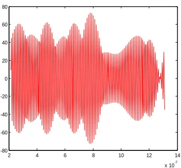
[image:4.595.69.257.82.281.2]The filter‟s output is shown in Fig. 10 and Fig. 11. The first thing to notice is the delay of approximately 2*10-7 produced by the filtering process. Besides this delay, the filtering performs as expected since we are left with only the baseband spectrum. We must recall that subcarriers 853 to 1705 are located at the right of 0 Hz, and the subcarriers 1 to 852 are to the left of 4 Hz. The next step is to perform the quadrature amplitude modulation(QAM) of the signal named UOFT in Fig. 3. In this modulation, an in phase signal and a quadrature signal are modulated.
0 0.2 0.4 0.6 0.8 1 1.2 x 10⁻⁶ -100
-50 0 50 100
0 0.2 0.4 0.6 0.8 1 1.2 x 10⁻⁶ -100
-50 0 50
0 0.5 1 1.5 2 2.5 3 3.5 4
x 108 0
20 40 60
0 50 100 150 200 250 300 350
-150 -100 -50 0
Frequency (MHz)
P
o
w
e
r/
fr
e
q
u
e
n
c
y
(
d
B
/H
z
) Welch Power Spectral Density Estimate
Figure.8 Frequency response of signal U
0 0.2 0.4 0.6 0.8 1 1.2 1.4 1.6 1.8 2 x 10⁸ -700
-600 -500 -400 -300 -200 -100 0 100
Figure.9 D/A filter response
2 4 6 8 10 12 14
x 10-7 -100
-50 0 50 100
2 4 6 8 10 12 14
x 10-7 -100
[image:4.595.78.257.329.440.2]-50 0 50
Figure.10 Time response of the filter output (UOFT)
0 0.5 1 1.5 2 2.5 3 3.5 4 x 10⁸ 0
20 40 60
-100 -50 0
eq
ue
nc
y
(d
B
/H
z)
[image:4.595.322.538.329.583.2] [image:4.595.81.254.607.719.2] [image:4.595.327.534.627.740.2]2 4 6 8 10 12 14
x 10-7 -80
-60 -40 -20 0 20 40 60 80
Figure.12 Time response of the ouput signal s(t)
0 0.5 1 1.5 2 2.5 3 3.5 4
x 108 0
10 20 30
0 20 40 60 80 100 120 140 160 180
-150 -100 -50 0
Frequency (MHz)
P
o
w
e
r/
fr
e
q
u
e
n
c
y
(
d
B
/H
z
[image:5.595.78.258.79.246.2]) Welch Power Spectral Density Estimate
Figure.13 Frequency response of the output signal s(t)
Table.1 Parameter values used in simulation
PARAMETER 2K mode
Elementary period T 7/64µs Number of carriers K 1705
Value of Kmin 0
Value of Kmax 1704
Duartion Tu 224µs
Carrier spacing 1/Tu 4464 Hz
Spacing between kmin and
Kmax(K-1)/Tu
7.61 MHz
Allowed guard interval ¼ 1/8 1/16 1/32
Duration of Tu 224µs
Duration of guard interval 56µs 28 µs 14 µs 7 µs
Symbol Duration 280µs 252µs 238µs 231 µs
4.2
DVB-T RECEPTION
The design of an OFDM receiver is open. For example, the frequency sensitivity drawback is mainly a transmission channel prediction issue ,something that is done at the receiver ;therefore, we shall only present a basic receiver structure in this report.OFDM is very sensitive to timing and frequency offsets[7]. Even in this ideal simulation environment, we have to consider the delay produced by the filtering operation. For our simulation, the delay produced by the reconstruction and demodulation filters is about TD=64/RS. This delay is enough to impede the reception, and it is
[image:5.595.310.576.271.416.2]the cause of the slight differences we can see between the transmitted and received signals. With the delay taken care of, the rest of the reception process is straightforward. As in the transmission case, we specified the names of the simulation variables and the output processes in the reception description of Fig.14 shown below.
Figure 14: OFDM reception
The results of this simulation are shown in Fig.15 to Fig.22.
0 0.2 0.4 0.6 0.8 1 1.2 x 10⁻⁶ -50
0 50
0 0.2 0.4 0.6 0.8 1 1.2 x 10⁻⁶ -100
[image:5.595.69.258.296.491.2]-50 0 50 100 150
Figure.15 Time response of signal r_tilde
0 0.5 1 1.5 2 2.5 3 3.5 4
x 108 0
10 20 30
0 50 100 150 200 250 300 350
-150 -100 -50 0
Frequency (MHz)
P
o
w
e
r/
fr
e
q
u
e
n
c
y
(
d
B
/H
z
[image:5.595.341.512.463.740.2]) Welch Power Spectral Density Estimate
Figure.16 Frequency response signal of r_tilde
a_hat r_data
r_info
LP F
F
S=2
/T
4096
FFT
4- QA M Slice
r r_tilde
[image:5.595.48.290.563.754.2]Volume 44– No.22, April 2012
0 0.2 0.4 0.6 0.8 1 1.2
x 10-6 -50
0 50
0 0.2 0.4 0.6 0.8 1 1.2
x 10-6 -100
[image:6.595.64.265.64.766.2]-50 0 50 100 150
Figure.17 Time response of signal r_info
0 0.5 1 1.5 2 2.5 3 3.5 4 x 10⁸ 0
20 40 60
0 50 100 150 200 250 300 350 -150
-100 -50 0
Frequency (MHz)
P
ow
er
/f
re
qu
en
cy
(
dB
/H
z) Welch Power Spectral Density Estimate
Figure.18 Frequency response signal r_info
0 0.2 0.4 0.6 0.8 1 1.2 x 10⁻⁶ -50
0 50
0 0.2 0.4 0.6 0.8 1 1.2 x 10⁻⁶ -100
-50 0 50 100 150
Figure.19 Time response of signal r_data
0 0.2 0.4 0.6 0.8 1 1.2 1.4 1.6 1.8 2 x 10⁷
0 0.5 1 1.5
0 2 4 6 8 10 12 14 16 18 -100
-80 -60 -40 -20
Frequency (MHz)
P
ow
er
/f
re
qu
en
cy
(
dB
/H
z)
Welch Power Spectral Density Estimate
Figure.20 Frequency response of signal r_data
-0.4 -0.2 0 0.2 0.4 0.6 0.8 1
info-h Received Constellation
-1.5 -1 -0.5 0 0.5 1 1.5 -1.5
-1 -0.5 0 0.5 1 1.5
[image:6.595.325.537.70.176.2]ahat 4-QAM
Figure.22 a_hat constellation
5.
CONCLUION
The transmission and the reception model have been discussed in details along with their Welch power spectral density estimation. For each step their time domain signal and also their frequency domain signal has been plotted. For the power spectral density estimation we used the Welch method rather than the Bartlett method as it cuts down on the noise factor. This whole paper is based on the simulation results obtained from the simulation of DVB-T signal using the 2K mode and the parameters specified for the same. Further studies are being done in order to compare the obtained results with the 8K mode of DVB-T.
6.
ACKNOWLEDGEMENT
We would like to thank Mr. Chandika Mohan Babu, our guide, and Mrs. Vinit Dhaliwal, our COD, and our teacher Ms. Ria Kalra for helping us in doing this research paper. Without their help this would not have been a success.
7.
REFERENCES
[1] A. Yiwleak and C. Pirak, “Intercarrier Interference Cancellation Using Complex Conjugate Technique for Alamouti-Coded MIMO-OFDM Systems” In Proceeding of International conference on Electrical Engineering/ElectronicsComputer Telecommunications and Information Technology no. 5, pp-1168-1172,
(Chaing Mai) 2010.
[2] C. Yuen, Y. Wu, and S. Sun, “Comparative study of
open-loop transmit diversity schemes for four transmit antennas in coded OFDM systems,” In Proceeding of IEEE conference on Vehicular Technology, pp. 482–485, (Baltimore, MD)September 2004
[3] A. Boariu and D.M. Ionescu “A class of nonorthogonal
rate-one space time block codes with controlled interference,” IEEE Transactions on Wireless Communications, Vol. 2, Issue 2, pp. 270–395, March 2003
[4] V. Tarokh, H. Jafarkhani and A. R. Calderbank, “Space– time block codes from orthogonal designs”, IEEE Transactions on Information Theory, Vol. 45, pp. 1456– 1467, July 1999
[5] J. Kim and I. Lee, “Space–time coded OFDM systems
with four transmit antennas,” In Proceeding of IEEE conference on Vehicular Technology, vol. 2, pp. 2434– 2438, September 2004.
[6] Orthogonal frequency division multiplexing for high-speed optical transmission, by Ivan B. Djordjevic et al
[7] A Novel Construction Technique For Designing Of Video Application Using Wirless 4G, by M.Suman et al.
[8] Comparison of OFDM, SC-FDMA and MC-CDMA as AccessTechniques for Mobile Communication, by Zohaib Shaikh et al.
[9] OFDM Simulation Using Matlab,
[image:6.595.82.253.83.249.2]