F U L L P A P E R
Open Access
Ionospheric current contribution to the main
impulse of a negative sudden impulse
Geeta Vichare
*, Rahul Rawat, Ankush Bhaskar and Bashir M Pathan
Abstract
The geomagnetic field response to a moderate-amplitude negative sudden impulse (SI−) that occurred on 14 May 2009 at 10:30 UT was examined at 97 geomagnetic observatories situated all over the globe. The response signature contains a contribution from magnetospheric as well as ionospheric currents. The main impulse (MI) is defined as the maximum depression in the observed geomagnetic field. It is observed that for low-to-high latitudes, the amplitude of the MI is larger in the afternoon to post-dusk sector than in the dawn-noon sector, indicating asymmetry in the MI amplitude. We estimated the contribution at various observatories due to the Chapman-Ferraro magnetopause currents using the Tsyganenko model (T01) and subtracted this from the observed MI amplitude to obtain the contribution due to ionospheric currents. It is found that the ionospheric currents contribute significantly to the MI amplitude of moderate SI−even at low-to-mid latitudes and that the contribution is in the same direction as that from the magnetopause currents near dusk and in the opposite direction near dawn. The equivalent current vectors reveal a clockwise (anticlockwise) ionospheric current loop in the afternoon (morning) sector during the MI of the negative pressure impulse. This evidences an ionospheric twin-cell-vortex current system (DP2) due to field-aligned currents (FACs) associated with the dusk-to-dawn convection electric field during the MI of an SI−. We also estimated the magnetic field variation due to prompt penetration electric fields, which is found to be very small at low latitudes in the present case. The studied SI− is not associated with shock, and hence no preliminary reverse impulse was evident. In addition, the summer hemisphere reveals larger MI amplitudes than the winter hemisphere, indicating once again the role of ionospheric currents.
Background
A sudden enhancement/drop in solar wind dynamic pressure causes the sudden compression/expansion of the magnetosphere, forming a positive/negative sudden impulse (SI) in the geomagnetic field (Nishida and Jacobs 1962). The signatures of these impulses in the ground magnetic field are quite complex due to the con-tributions from several current systems flowing in the magnetosphere and ionosphere. Using rapid-run magne-tograms, it has been observed that the geomagnetic re-sponse signature of an SI is preceded by an initial rapid variation. The broad features of the geomagnetic signa-ture include a first rapid response, also known as a pre-liminary impulse (PI) with a time scale of a few seconds to a few minutes, followed by a main impulse (MI). Araki (1977) described the geomagnetic signature of SIs
in terms of a preliminary impulse of polar origin (DPpi), a main impulse dominating at low latitude (DLmi), and a main impulse of polar origin (DPmi). The PI is further categorized into positive and negative PIs. If the PI is negative (positive) during enhanced (reduced) solar dy-namic pressure, then it is known as a preliminary re-versed impulse (PRI). The DL field is a stepwise change in the geomagnetic field, and the DP field is a bipolar type. In this paper, we define the MI of a negative SI as the maximum reduction in the total field containing DPpi, DLmi, and DPmi parts.
Over the past six decades, several studies have been dedicated to understanding the characteristics of SIs (Sugiura 1953; Nagata and Abe 1955; Matsushita 1962; Sano 1962; Tamao 1964; Nishida et al. 1966; Rastogi and Sastri 1974; Araki et al. 1985, 2006; Araki and Nagano 1988; Araki 1994; Sastri et al. 1995; Yamada et al. 1997; Takeuchi et al. 2000, 2002a; Villante and Di Giuseppe 2004; Huang et al. 2008; Shinbori et al. 2009; Wang et al. 2009). Based on the magnetic field observations on
* Correspondence:[email protected]
Indian Institute of Geomagnetism, New Panvel, Navi Mumbai, Maharashtra 410218, India
ground, an equivalent ionospheric current system for the PI has been deduced (Araki et al. 1985; Araki 1994), which is similar to the DP2 current system (Nishida et al. 1966). This current system consists of twin-vortex type ionospheric currents generated by field-aligned cur-rents (FACs) that give a bipolar signature on the ground (Araki 1994). The MI signature mainly comprises contri-bution due to currents flowing at the magnetopause and transient currents generated in the ionosphere and mag-netosphere. Rastogi and Sastri (1974) found that the equatorial enhancement is larger for a PRI than for an MI, highlighting the stronger role of ionospheric con-ductivity in a PRI than that during an MI. Attempts have been made to study the local time (LT) variation of MI amplitude; for example, Shinbori et al. (2009) studied this variation statistically. However, not many studies have been carried out to investigate the LT variation for an individual SI. Gaining an understanding of this is important, as the results may differ for various SI events because the geomagnetic field response to SIs strongly de-pends on factors such as the orientation and magnitude of the interplanetary magnetic field (Wing and Sibeck 1997; Lee and Lyons 2004), orientation of shocks/discontinuities (Takeuchi et al. 2002b; Wang et al. 2006), the value of pressure before disturbance, and the change in pressure amplitude (Borodkova et al. 2006). Therefore, any statis-tical studies performed without consideration of these as-pects may be unable to provide a true picture of the LT variation, which indicates the importance of case studies.
It has been estimated that the time required for a plasma front to sweep past the geomagnetic field is not more than 30 s, but the observed rise time of SIs is a few minutes. According to the model presented by Dessler et al. (1960), a negative correlation between SI amplitude and rise time can be expected because the larger the dis-tance of the SI source from the observer, the longer the rise time and the smaller the amplitude due to attenu-ation. The time duration of SI depends on the following: the time taken by the shock front or discontinuity to sweep the geoeffective distance along the magnetosphere, the thickness of the shock front or the discontinuity in the solar wind, inertia of the magnetospheric plasma, and the broadening of the wave front during the passage through the magnetosphere (Nishida 1966). Wang et al. (2006) sta-tistically investigated the effect of the interplanetary shock strength and orientation on SI rise time and found that oblique shocks result in a longer rise time of SIs.
Nishida and Jacobs (1962) noticed a similarity between positive and negative SIs and claimed that any theory of positive impulse (SI+) should be able to explain the
phenomenon of negative impulse (SI−) in an opposite
sense. In support of this, several studies investigating geomagnetic field response to the negative solar dynamic pressure pulses reported that the response is opposite to
that of the positive impulse (Rastogi and Sastri 1974; Araki and Nagano 1988; Sastri et al. 1995; Takeuchi et al. 2000), which indicated that negative SIs can be explained by the physical model used for positive impulses but with reversed current systems. The numerical simulation of a
moderate amplitude SI−using solar
wind-magnetosphere-ionosphere MHD model by Fujita et al. (2004) showed that the SI− is basically a mirror image of the SI+. How-ever, Fujita et al. (2012) later revisited the simulations with larger amplitude SI− and concluded that SI−and SI+ are not in a mirror image relation. They listed a few differ-ences between SI− and SI+, such as the overshielding of the convection electric field occurring in the MI phase of a negative SI event and in the PI phase of SI+, but the dur-ation of the shielding for SI+ being shorter than that for
the SI−. Using SuperDARN data, Hori et al. (2012)
ob-served differences in the ionospheric flow during SI− and SI+, and Takeuchi et al. (2000, 2002a) also reported that the polarization distribution of SI−is not opposite to that of SI+. Thus, various studies carried out during the last decade have pointed out differences between positive and
negatives SIs, and have demonstrated that an SI− is not
simply mirror image of an SI+.
Tamao (1964) proposed the mechanism of an equiva-lent current system for a PRI, based on the three-dimensional propagation of hydromagnetic waves in cold plasma, whereas Kikuchi and Araki (1979) proposed the Earth-ionosphere waveguide TM0 mode as a mechanism of propagation of polar electric fields to the equator and applied this to the PRI occurrence at the equator. Tamao (1964) model suggested that the direct source of the PRI is an ionospheric Hall-current system caused by the inci-dence of mixed transverse hydromagnetic waves (pure transverse plus converted transverse), and Chi et al. (2001) observed a very good agreement between the ob-served rise time of the PRI and the rise time calculated
using Tamao’s (1964) model. However, according to
Kikuchi and Araki (2002), Tamao’s (1964) model cannot
be applied at low latitudes because the rotational electric fields of the converted transverse mode do not generate the Hall currents that close in the ionosphere. They also pointed out that the Hall currents accompany the Peder-sen currents in a collision-dominated ionosphere, and therefore the energy dissipated by the Pedersen currents could not be supplied by the converted transverse mode. Therefore, although both models predict and explain a few features of an SI, it appears that a more detailed in-vestigation is required to resolve the issues described above.
This paper is presented as follows: firstly in ‘Database’ section, we introduce the event of a negative solar wind pressure impulse along with other solar wind and interplanetary parameters. ‘Observation’ section presents the response to the SI−at geosynchronous satellites and at various ground observatories, and‘Results and discussion’ section describes the characteristics of the SI−, such as the contribution due to sudden changes in IMF, local time variation of the MI amplitude and duration, equivalent ionospheric currents during the MI phase, latitudinal vari-ation of MI amplitude, hemispheric asymmetry, and the geomagnetic response after attaining maximum depres-sion. Finally,‘Conclusions’section discusses and summa-rizes the findings of the present investigation.
Methods
Database
This study utilized 1-min time resolution geomagnetic data downloaded from the INTERMAGNET website
(http://www.intermagnet.org). Digital fluxgate data
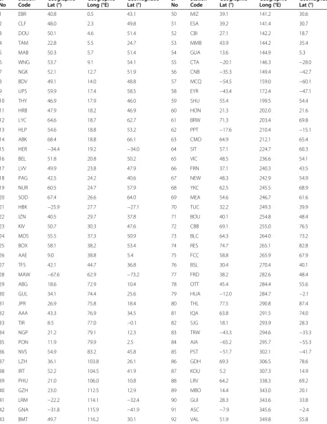
with a 1-min resolution from the World Data Center of Geomagnetism, Kyoto and from a chain of observator-ies in the Indian longitude zone were also used. Table 1 lists the observatories along with their geographic latitude and longitude and geomagnetic latitudes. In addition to ground magnetic observations, magnetic data from geo-synchronous satellites GOES-10, GOES-11, and GOES-12 were utilized.
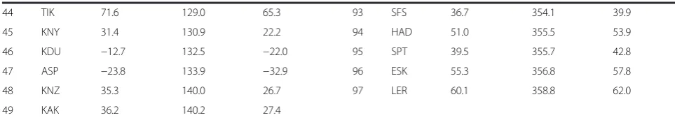
The event analyzed in this study was associated with moderate solar wind density variations accompanied by sudden changes in the orientation of the interplanet-ary magnetic field (IMF). Figure 1 shows the solar wind (SW) and IMF parameters on 14 May 2009 between 10:00 and 17:00 UT. The IMF and solar wind data from the ACE satellite were downloaded from http://spidr.ngdc. noaa.gov and are displayed in the figure without correc-tion for travel time delay. The solar wind number density dropped suddenly at 10:40 UT from 7/cc to 1/cc within 4 min, and the corresponding change in SW dynamic pressure was−1.41 nPa, a change of about 93%. It is im-portant to note that before the drop, the SW density was not steady but was oscillating. The density drop took place in two steps: at the end of the sudden decrease, there was a small gap in the SW density data followed by a slight in-crease, and the density then remained almost constant until 15:15 UT when the sudden density enhancement
took place. Thus, the present SI−event was accompanied
by an SI+event.
A statistical study by Takeuchi et al. (2002a) reported that 50% of SI− events occur in tandem with SI+ events. They found that interplanetary reversed shocks are not a primary cause of SI−events. Instead, SI−events are pro-duced by rapid decreases in the solar wind dynamic pres-sure associated with a variety of interplanetary structures
such as tangential discontinuities at high-low speed stream interfaces within co-rotating interaction re-gions (CIRs), the front boundaries of magnetic clouds, the rear boundaries of non-compressive density enhance-ments (NCDEs), the front boundary of a small-scale plasma hole, and earthward propagating shocks from the rear side of a solar flare (Takeuchi et al. 2002b; Rastogi et al. 2010). Takeuchi et al. (2002a) identified a pair of
SI−-SI+ associated with a small-scale plasma hole
em-bedded in a CIR, close to a heliospheric current sheet (HCS) and parallel to the Parker spiral direction.
In the present case, the southward component of the interplanetary magnetic field (IMF Bz) suddenly turned northward during a negative impulse and then remained constant until a positive enhancement of the SW density took place, where IMF Bz rapidly turned southward. In addition, the negative and positive impulses were accom-panied by sudden turnings of the X and Y components of the IMF. The magnetic pressure of SW remained high between SI− and SI+, with discernible discontinuities at the edges. The interplanetary structure seems, therefore, to be bounded by tangential discontinuities. These charac-teristics of the IMF and the SW parameters may indicate that a cavity with a low-particle density was impinging on the Earth's magnetosphere. The scale length of the discon-tinuity appeared to be about 5.6 × 10⁶km. Using magnetic co-planarity, the orientation of the discontinuity (the angle between the discontinuity normal and the GSEX-axis) is estimated (Schwartz 1998) and was found to be parallel to the Parker spiral at 1 AU.
The bottom plot in Figure 1 depicts the SYM-H index that indicates a sudden drop at approximately 12:00 UT associated with a negative pressure pulse and an increase at 16:30 UT corresponding to a positive impulse. The
MI signature during the SI− is shown between the two
vertical lines in the SYM-H plot. The amplitude of the
negative impulse in the SYM-H is around −27 nT. The
Table 1 List of geomagnetic observatories
Sr No
Station Code
Geographic Lat (°)
Geographic Long (°E)
Geomagnetic Lat (°)
Sr No
Station Code
Geographic Lat (°)
Geographic Long (°E)
Geomagnetic Lat (°)
1 EBR 40.8 0.5 43.1 50 MIZ 39.1 141.2 30.6
2 CLF 48.0 2.3 49.8 51 ESA 39.2 141.4 30.7
3 DOU 50.1 4.6 51.4 52 CBI 27.1 142.2 18.7
4 TAM 22.8 5.5 24.7 53 MMB 43.9 144.2 35.4
5 MAB 50.3 5.7 51.4 54 GUA 13.6 144.9 5.3
6 WNG 53.7 9.1 54.1 55 CTA −20.1 146.3 −28.0
7 NGK 52.1 12.7 51.9 56 CNB −35.3 149.4 −42.7
8 BDV 49.1 14.0 48.8 57 MCQ −54.5 159.0 −60.1
9 UPS 59.9 17.4 58.5 58 EYR −43.4 172.4 −47.1
10 THY 46.9 17.9 46.0 59 SHU 55.4 199.5 54.4
11 HRB 47.9 18.2 46.9 60 HON 21.3 202.0 21.6
12 LYC 64.6 18.7 62.7 61 BRW 71.3 203.4 69.8
13 HLP 54.6 18.8 53.2 62 PPT −17.6 210.4 −15.1
14 ABK 68.4 18.8 66.1 63 CMO 64.9 212.1 65.4
15 HER −34.4 19.2 −34.0 64 SIT 57.1 224.7 60.3
16 BEL 51.8 20.8 50.2 65 VIC 48.5 236.6 54.1
17 LVV 49.9 23.8 47.9 66 FRN 37.1 240.3 43.5
18 PAG 42.5 24.2 40.6 67 NEW 48.3 242.9 54.9
19 NUR 60.5 24.7 57.9 68 YKC 62.5 245.5 68.9
20 SOD 67.4 26.6 64.0 69 MEA 54.6 246.7 61.6
21 HBK −25.9 27.7 −27.1 70 TUC 32.2 249.3 39.9
22 IZN 40.5 29.7 37.8 71 BOU 40.1 254.8 48.4
23 KIV 50.7 30.3 47.6 72 CBB 69.1 255.0 76.5
24 MOS 55.5 37.3 50.9 73 BLC 64.3 264.0 73.2
25 BOX 58.1 38.2 53.4 74 RES 74.7 265.1 82.8
26 AAE 9.0 38.8 5.4 75 FCC 58.8 265.9 67.9
27 TFS 42.1 44.7 36.8 76 BSL 30.4 270.4 40.1
28 MAW −67.6 62.9 −73.2 77 FRD 38.2 282.6 48.4
29 ABG 18.6 72.9 10.4 78 OTT 45.4 284.4 55.6
30 GUL 34.1 74.4 25.6 79 HUA −12.0 284.7 −2.1
31 JPR 26.9 75.8 18.4 80 THL 77.5 290.8 87.4
32 AAA 43.3 76.9 34.5 81 IQA 63.8 291.5 74.0
33 TIR 8.5 77.0 −0.1 82 SJG 18.1 293.9 28.3
34 NGP 21.2 79.1 12.3 83 TRW −43.3 294.6 −33.3
35 PON 11.9 79.9 2.5 84 AIA −65.2 295.7 −55.3
36 NVS 54.9 83.2 45.8 85 PST −51.7 302.1 −41.7
37 LZH 36.1 103.8 26.1 86 GDH 69.3 306.5 78.6
38 IRT 52.2 104.5 41.9 87 KOU 5.2 307.3 14.9
39 PHU 21.0 106.0 10.8 88 LRV 64.2 338.3 69.2
40 GZH 23.0 112.5 12.9 89 MBO 14.4 343.0 20.1
41 LRM −22.2 114.1 −32.4 90 GUI 28.3 343.6 33.8
42 GNA −31.8 115.9 −41.9 91 ASC −7.9 345.6 −2.4
is also observed that 3-h kp values during the interval did not rise above the value of 3.
Observations
Magnetospheric response
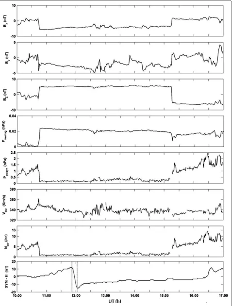
Magnetic field variations in the geosynchronous orbit are plotted in Figure 2, where magnetic data with a 1-min resolution from three satellites (GOES-10, GOES-11, and GOES-12) was available during the event. At the time of the event, magnetic local times (MLT) were approxi-mately 03:00, 07:00, and 08:00 at GOES-11, GOES-12, and GOES-10, respectively. Figure 2 shows all three com-ponents of the magnetic field (Hp, He, and Hn) and the magnitude of the total magnetic field vector (Ht). From Figure 2, it can be seen that the variation in the Hp com-ponent associated with the SI dominates over the other components during the daytime, while GOES-11 (located at 03:00 MLT) records comparable SI-related variations in all three components. The magnetic field variations due to the sudden solar wind pressure changes at the geosynchronous orbit are mainly of the compressional or rarefactional type and are represented by the Hp com-ponent (Wang et al. 2009). We therefore only discuss the Hp component of the magnetic field here. The response signature at a geosynchronous height is essentially a simple step-like decrease, and the amplitudes of the sud-den negative impulse at 03:00, 07:00, and 08:00 MLT
are −8, −19, and −25 nT, respectively. Thus, the
mag-nitude increases during daytime, which is consistent with earlier observations at geosynchronous orbit (Kokubun 1983) and could be attributed to larger changes in the magnetopause currents at a sub-solar point (Villante and Piersanti 2011).
Two features can be observed that occurred before the onset of the event at all three satellites: a gradual in-crease in the magnetic field and wavy structures. The fluctuating structures at GOES-12 and GOES-10 (both located in the nearby MLT zone in the morning hours) are similar, while those of GOES-11 (3:00 MLT) shows damped fluctuations, indicating daytime enhancement of the wavy structures. These observations can be attrib-uted to the fluctuations riding on the steady increase of the solar wind dynamic pressure observed prior to the SI−impulse (Figure 1).
As the ground magnetic observatory at Huancayo lies on the same meridian and equatorial plane as the GOES-12 satellite, we compare the magnetic field re-sponses at these two locations. The amplitude of the MI
at the HUA station is larger (approximately −50 nT)
than at GOES-12 (approximately−19 nT), and the
amp-litude ratio of the satellite to the ground is 0.34, which is moderately smaller than that recorded by Kokubun (1983) (0:55 at 07:00 MLT). The fall time during a nega-tive impulse at GOES-12 is approximately 6 min, which is longer than the SW density impulse duration (4 min) and shorter than that on the ground (approximately 11 min in SYM-H).
Ground-based observations
Figure 3a,b,c,d,e,f,g,h displays the horizontal field re-sponse to sudden magnetospheric rarefaction in various longitudinal sectors, for a period of 50 min from 11:40 to 12:30 UT on 14 May 2009, corresponding to local times ranging from 02:00 to 22:00. Each sub-figure shows a stacked plot of H-variations at different geomagnetic latitudes (displayed on the right side), and quiet time variations at each station are plotted in the background. Almost all the stations reveal a stepwise decrease in the horizontal component of the geomagnetic field (H). As SYM-H can be roughly considered representative of the average geomagnetic response, the onset time of the nega-tive pressure impulse is determined from SYM-H index and is shown by vertical lines at 11:50 UT in Figure 3. Figure 3a displays four plots in the longitude belt between 210°E and 240°E that correspond to 02:10 to 04:10 MLT, and the geomagnetic latitudes of the stations in this longi-tude sector are 65°N, 60°N, 54°N, and 15°S. Note that in Figure 3a,b,c,f, the scales of the H amplitudes are different for high and mid-to-low latitudes. An examination of the response in various local times and latitudinal sectors shows a disparity in the response signature. Some of the plots show a small positive increase near the onset time (e.g., the polar stations in Figure 3b,c and at a few high-to-middle latitude stations in Figure 3d,e,f), which may indi-cate the occurrence of a PRI signature. While some plots show no initial increase (e.g., the plots in Figure 3a,g,h), some plots show a sudden drop with a very smooth de-crease (Figure 3a,g,h), and in some plots this drop has a Table 1 List of geomagnetic observatories(Continued)
44 TIK 71.6 129.0 65.3 93 SFS 36.7 354.1 39.9
45 KNY 31.4 130.9 22.2 94 HAD 51.0 355.5 53.9
46 KDU −12.7 132.5 −22.0 95 SPT 39.5 355.7 42.8
47 ASP −23.8 133.9 −32.9 96 ESK 55.3 356.8 57.8
48 KNZ 35.3 140.0 26.7 97 LER 60.1 358.8 62.0
wavy structure. As stated in the‘Background’section, we refer to the sudden drop (or the duration from onset to maximum reduction) as the phase of the MI.
It can be observed from Figure 1 that the decrease in the solar wind pressure took place in two steps. At certain locations, particularly where an initial positive variation (just after the onset) is observed, two clearly discernible steps are observed in the MI. It is possible that the initial positive type of variation prior to the second step separates the MI signature of the second negative impulse from that of the first impulse, result-ing in two discrete MI signatures. Stations with no initial positive signature show a smooth decrease in the H com-ponent which could be due to MI signatures only as-sociated with the two consecutive negative impulses. Therefore, in general, the wavy signatures seen at cer-tain locations during the MI phase of a two-step negative impulse may suggest the existence of an initial positive signature.
There is another aspect associated with the fluctua-tions observed before the onset and during the MI. Note that in Figure 3, some of the plots show oscillating struc-tures before the onset time while other plots show no such fluctuations (e.g., plots in Figure 3g,h). As noted in Figure 1, the SW pressure was already oscillating before the sudden drop took place, and it is therefore possible that these oscillations are seen in the ground data. Interestingly, these oscillations are prominently observed
during the daytime. In addition, when there is an absence of oscillations during an MI, there is also generally an ab-sence of oscillations before the onset.
Also note that after the minimum, the geomagnetic field shows a positive variation in general and then tries to attain steady state. This variation after the maximum depression is also different at different locations and local time sectors.
Geomagnetic latitudinal belt between 40°N and 50°N Figure 3 shows that the geomagnetic response to the SI− varies with latitude and local time. In order to examine the LT variations of the response, we choose a narrow range of latitude between 40° and 50°, where a good num-ber of stations were available. Figure 4 shows the stacked plots of D- (left-hand panel) and H- (right-hand panel) variations recorded at observatories essentially between the geomagnetic latitudes of 40°N and 50°N, although a couple of observatories that lie just outside this latitudinal range are also included. The MLTs at each station are dis-played on the right side of the figure, and the plots are ar-ranged with increasing MLT from bottom to top. As noticed in the previous sub-section, the geomagnetic field response to SI−at certain locations has an initial positive variation, which may indicate the occurrence of PRI. How-ever, the PRI has a very rapid and strong variation that only lasts a few seconds. It is possible that the 1-min time-averaged values used in the present analysis may not have (See figure on previous page.)
Figure 1Solar wind and IMF parameters on 14 May 2009 between 10:00 and 17:00 UT.Bx, By, and Bz are interplanetary magnetic field components;PSWmagandPSWdynare magnetic and dynamic pressures of the solar wind, respectively;VSWandNSWare the velocity and density of the solar wind recorded by ACE satellite (all parameters are displayed without correction for travel time delay). Bottom plot shows SYM-H index where the MI of the negative impulse is shown between two vertical lines.
been able to display larger variations of smaller time scales. Therefore, in this section, we depict 1-s values of the geo-magnetic field at a few available stations, as highlighted by the blue color in the figure. We use five stations (FRD,
1-s data do not evidence a clear intense enhancement in the amplitude of the positive increase. Therefore, it is not possible to confirm that the initial positive variation represents the PRI signature, and hence it is not possible to infer about the occurrence of the PRI.
The D-variations (expressed in nanotesla) in the four lowest plots in the left-side panel with MLTs between 03:30 and 06:41 show an initial increase after the onset time, and thereafter a decrease. At 07:52 MLT, the southern hemispheric station PST shows a very small D-variation, and the stations beyond this MLT show a positive type of MI signature in the D component. Few stations show an initial very small decrease followed by an increase. The signature of the main impulse in the D component is ob-served to be negative after midnight to near dawn and positive from afternoon to post-dusk.
Response waveforms in the H and D components show noticeable variations after the main impulse signature. The geomagnetic response signature in the H compo-nent shows a positive variation in general after achieving the minimum and then tries to attain a quasi-steady state. We call the first variation occurring immediately
after the minimum the ‘after maximum deviation’
(AMD) variation. In actual fact, one more oscillation appears at a few stations after this variation, but it has a very weak amplitude. Similarly in the D component, a signature opposite to the main impulse is observed just after the maximum deviation. To define the various phases of the response waveform, we indicate points d1, d2, d3, h1, h2, and h3 in the topmost plots of Figure 4. The points indicated by a subscript 1 show the onset time, which is also indicated by a vertical dashed line, and is assumed to be same for all the plots. Points with subscripts 2 and 3 indicate the end of the MI and AMD, respectively.
The amplitude of the MI is defined as the maximum deviation of the magnetic field from its pre-SI value. Hence, the MI amplitude in the H component is the vari-ation in the H component from the onset time to the time where H attains the minimum value (the H-variation roughly attains the minimum at approximately 11 to 13 min after the onset time). If the times at points h1, h2, and h3 are th1, th2, and th3, respectively, then the quan-tity defined by (H(th2)−H(th1)) represents the MI ampli-tudes in H. Similarly, if the times at points d1, d2, and d3 are td1, td2, and td3 respectively, then the quantities
defined by (D(td2)−D(td1)) represent the MI
ampli-tudes in the D component. The amplitude difference be-tween points 2 and 3 gives the amplitude of the AMD, i.e., (H(th3)−H(th2)) and (D(td3)−D(td2)). The MI amp-litude in the H-component is minimum
(approxi-mately −7 nT) near dawn and thereafter continues to
increase throughout the afternoon sector, reaching a
max-imum (approximately−47 nT) near dusk (at 18:54 MLT).
Low-latitude region (between 10° and 40° geomagnetic latitude)
At low latitudes, the geomagnetic field response to the solar wind pressure change is often step-like due to the Chapman-Ferraro magnetopause currents and a propagat-ing compressional wave front. Geomagnetic variations at low latitudes can be considered as remote to field-aligned, auroral ionospheric, and equatorial electrojet currents (Araki 1977, 1994). It has been found that a geomagnetic SI at low latitudes is proportional to the change of the square root of the solar wind pressure. Siscoe et al. (1968), Russell et al. (1994), and Takeuchi et al. (2002a) reported that the slope of the regression line is consistent during SI+ and SI− events.
In this section, we investigate the geomagnetic re-sponse in the low-to-mid latitude region between 10° and 40° geomagnetic latitude by plotting the MLT vari-ation of the MI amplitude in the H component (Figure 5). Note that in order to obtain sufficient MLT coverage, the low-latitude range is been widened up to 40°. As stated in the previous sub-section, the amplitude of
the MI is defined as ΔH=H(th2)−H(th1), where th1
is the onset time of SI and th2 is the time when the amplitude of the SI attains its maximum negative value. Note that if more than one station is available at a given MLT, then the average of the amplitudes at those stations is used to represent the amplitude of the MI at that particular MLT. Figure 5 depicts the higher MI ampli-tude of the negative impulse in the afternoon to
post-dusk sector (approximately −30 nT) and the minimum
near dawn (approximately −10 nT), exhibiting a strong
dawn-dusk asymmetry. According to the empirical
formula derived by Russell et al. (1994), ΔH¼k
ffiffiffiffiffiffiffiffiffi
, the change in the H component during
the presently studied negative impulse is around −16 nT
during daytime (k= 18.4 nT/nPa1/2), and
approxi-mately −13.3 nT at nighttime (k= 14.9 nT/nPa1/2). Note that these estimates are simple approximate values used for the comparison, although the actual magnetic field variations at each location due to magnetopause currents
are estimated in‘MLT dependence of ionospheric current
contribution in the MI amplitude’section using an empir-ical model. The departure of the observed MI magnitude from these rough values can be due to the contribution of other current systems that develop in the magneto-spheric and ionomagneto-spheric domain during SIs. In general, the amplitude of the response in the pre-dawn sector is comparable to that due to changes in the solar wind pressure, and the variation is almost double due to a simple pressure impulse in the afternoon zone, suggest-ing an additional contribution from other transient cur-rents present during the event. A statistical study of SIs by Shinbori et al. (2009) showed that at low-to-mid latitudes, the amplitude attains a minimum at around 08:00 MLT, then increases towards noon, peaks in the afternoon hours, and once again peaks at midnight. Unfortunately, data between 22:00 and 00.00 MLT was not available in this latitudinal range, and hence we are unable to examine the nighttime enhancement of the H amplitude as reported by Araki et al. (2006) and Shinbori et al. (2009). However, from Figure 5 it is possible to observe that the H amplitude attains a minimum near 07:30 MLT and is fairly high at around 19:00 MLT; thus, the overall local time variation depicted in Figure 5 matches very well with that reported by Shinbori et al. (2009).
The differences in MI amplitude at dawn and dusk are quantified by defining the asymmetry index as
γ¼ MIdusk−MIdawn
MIduskþ MIdawn
where MIdawn (= −11 nT) and MIdusk(= −33 nT) are
the minimum and maximum values of MI amplitudes at
dawn and dusk respectively, which gives value ofγequal
to 0.5 in the present case. The dawn-dusk asymmetry index computed by Shinbori et al. (2009) for low lati-tudes up to 27° is around 0.2 and suddenly increases to approximately 1.2 at 35° latitude (Figure four in Shinbori et al. (2009)), and the average over 10° to 40° latitude is around 0.6, which compares well with our case study.
Equatorial region
In this section, we present observations at equatorial stations from different MLT sectors. A list of five equa-torial stations is displayed in Table 2 (geomagnetic
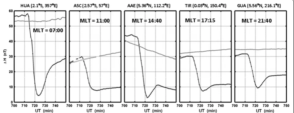
latitude < ± 6°), together with geographic longitude and geomagnetic and dip latitudes. Figure 6a,b,c,d,e displays the geomagnetic field variations at HUA, ASC, AAE, TIR, and GUA, and the background variations shown by the thin lines represent the quiet time variation at a given station. The MLTs at HUA, ASC, AAE, TIR, and GUA were 07:00, 11:00, 14:40, 17:15, and 21:40, respect-ively. It can be seen that there is a small positive vari-ation before the main negative impulse at HUA, while ASC, AAE, TIR, and GUA have a clear MI-type signa-ture without an initial positive increase. We examined the 1-s resolution data from the HUA observatory and noticed no remarkable enhancement in the amplitude of the initial positive variation. It is therefore difficult to comment on whether the initial positive variation is re-lated to PRI or it could be a part of the fluctuations seen in the SW density before the onset.
The amplitudes of MI at HUA, ASC, AAE, TIR, and GUA are 50, 23, 40, 23, and 23 nT, respectively. It is in-teresting to note that the amplitude of the MI at ASC, which is near magnetic noon (at 11:00 MLT), has an amplitude of much less than that at 07:00 MLT and at 14:40 MLT. However, this can be justified through the dip latitude of ASC, which is quite high (approximately 25° S), and hence it is located quite far from the dip equator and experiences very small ionospheric conduct-ivity compared to the equatorial Cowling conductconduct-ivity. While comparing the observations in a narrow belt of the equatorial zone, it is necessary to bear in mind that the Cowling conductivity gradients in the vicinity of the magnetic equator are very sharp, resulting in large amp-litude differences within a few degrees of latitude. The geomagnetic latitude of HUA is 2.1°N, which is closer to the geomagnetic equator than AAE (5.36°N GMlat). Shinbori et al. (2009) found that the daytime enhance-ment of the normalized SI amplitude at 5° away from the magnetic equator (GAM) has a peak amplitude of less than half the value of that is found close to the mag-netic equator (YAP). From their Figure one, at 07:00 MLT, YAP had a normalized amplitude of 1.5, which was comparable with that at near noon at GAM. It is therefore quite possible that the present observation of the larger MI amplitude at 07:00 MLT could be due to the fact that HUA is located closer to the geomagnetic equator than AAE. Thus, in view of the magnetic
Table 2 Equatorial magnetic observatories
Station name Station code Geographic longitude Geomagnetic latitude Dip latitude
Addis Ababa AAE 38.77°E 5.36°N 1.34°N
Tirunelveli TIR 77.8°E 0.03°N 0.4°N
Guam GUA 144.88°E 5.56°N 6.34°N
Huancayo HUA 285°E 2.1°S 0.28°N
latitudes of the observatories, the differences in the MI amplitudes could be due to the sharp latitudinal gradi-ents of Cowling conductivity in a narrow belt of the equatorial region. Further, the dip latitudes of HUA and TIR are almost same (both situated close to the dip equator) and are located near dawn and dusk respect-ively. A comparison of the MI amplitude at these two lo-cations reveals larger MI amplitude at the near-dawn station, HUA, than that at the near-dusk station, TIR.
Results and discussion
Contribution due to sudden changes in the IMF
If the SIs are accompanied with sudden changes in the IMF, then it is possible that other factors such as mag-netopause currents, FAC and ionospheric currents, effects associated with prompt penetration, and over-shielding could also contribute to the geomagnetic response during the sudden SW pressure changes. Takeuchi et al. (2000) studied an SI−, whereΔPsw=−6.44
of −26 nT in the geomagnetic response on the ground.
It should be remembered that for the present event,ΔPsw of −1.41 nPa Δ ffiffiffiffiffiffiffiPsw
p
¼−0:9 pffiffiffiffiffiffiffiffinPa
resulted in a vari-ation of−27 nT in SYM-H. This indicates that there is an inconsistency in the amplitude of the geomagnetic re-sponse in the two cases, as a smaller amplitude rere-sponse would be expected in our case due to a smaller change in the SW dynamic pressure. Also note that in both cases, there was a sudden northward turning of the IMF at the time of the sudden drop in the pressure. However, during the event studied by Takeuchi et al. (2000) on 13 May 1995, the IMF changed from a smaller value to a larger value of a northward IMF, while during the presently
studied case on 14 May 2009, the sudden northward turning was from a southward direction to a northward IMF Bz. Recently, Bhaskar and Vichare (2013) have statistically shown that during a northward turning, in addition to the overshielding effects associated with R2 FACs, the reduction in the southward component con-tributes to the negative variation in the H component at equatorial stations during daytime. Therefore, it may be possible that for the presently studied case, there was a stronger negative contribution existing in the same direction as that due to the magnetopause currents during daytime and which may therefore have re-sulted in a larger decrease of the H component. In order to examine this possibility, we obtained the equa-torial prompt penetration electric fields (PPE) from the
‘Real-time model of the Ionospheric Electric Fields’
(http://www.geomag.us/models/PPEFM/RealtimeEF.html). Figure 7 displays the PPE from the above-mentioned model at different LTs and clearly shows the presence of a westward electric field during daylight hours and an eastward electric field during the nighttime. Using ionospheric conductivity values from World Data Center (WDC), Kyoto, we estimated the magnetic field varia-tions associated with PPE at low latitudes, which was
found to be approximately −2 nT at 12:00 MLT. Thus,
the magnetic field contribution due to PPE is very small for this event. In addition, we examined the ASYM-H index during the event and found this to be very high, which could be due to the presence of ionospheric cur-rents (DP2) or the partial ring current associated with the FACs generated during the SI. Therefore, the differ-ence in the geomagnetic field response between the present and earlier cases could be due to ionospheric currents associated with the FACs.
MLT dependence of ionospheric current contribution in the MI amplitude
The magnetic field response to sudden SW pressure changes comprises contributions from the Chapman-Ferraro magnetopause currents, ionospheric currents (such as the Pedersen currents and Hall currents), and field-aligned currents (FACs). Using the Tsyganenko empirical model, T01 (Tsyganenko 2002a,b), we compute the magnetic field produced by the Chapman-Ferraro cur-rents at the location of each ground observatory. Figure 8a shows the MLT variation of the observed MI amplitude in the H component at the stations located between 60°S
residual fields essentially represent the contribution from the ionospheric currents and FACs. The model estimates of the contribution from the magnetopause currents attain a maximum near noon (Figure 8b), while the observed MI amplitude peaks near dusk (Figure 8a). Near dusk, the amplitude of the residual field is considerably larger than that due to Chapman-Ferraro current contribution and hence reveals the significance of the ionospheric currents and FACs. Note that near dawn, the observed MI ampli-tudes are slightly smaller than those due to the magneto-pause currents, resulting in small positive values of the residual fields. The contribution due to the FACs is sym-metrical at about noon and has the same direction as in
ionospheric current contribution is in the same direction as that of the magnetospheric currents near dusk, thereby enhancing the amplitude of the observed MI.
Equivalent current system during the MI
Figure 9 shows the equivalent current vectors during the MI of the negative impulse, which are derived from the residual magnetic field variations in the H and D components during the main impulse, at the magnetic observatories located between the north pole and 35°N geomagnetic latitude (concurrent circles are drawn at 15° spacing). The residual magnetic field is obtained by sub-tracting the magnetopause current contribution from the observed MI amplitude. Note that here we consider only those stations where there was a distinct MI signature in both H and D components. The current vectors indicate the presence of a counterclockwise vortex near dawn and a clockwise vortex in the afternoon sector, although the centers of both the loops are not apparent. Thus, Figure 9 clearly demonstrates a two-cell current system during the main impulse of the SI−.
Local time dependence of the time duration of the MI
The ‘time duration’ (or fall time) of the MI is the time interval between the onset time and the end of the MI (th2-th1). From Figure 4, it can be noted that the dur-ation of the MI changes with the local time, and hence in this section, we plot the LT variation of the duration
of the MI in the H component for all stations (Figure 10). We also estimate the MI duration using another method where instead of using the minimum in the H compo-nent, we take the intersection of the line fits before and after the minimum. Estimates from these two methods show a similar LT dependence. In general, the Figure 9Equivalent current vectors (red arrows) during the main impulse of SI−event on 14 May 2009.
scatter plot and the 2-h average curve (solid line) show smaller values of the MI interval during the daytime com-pared to the nighttime. This is in accordance with the observations by Ondoh (1963) who showed that the time duration of both positive and negative SIs is shorter in the daytime than in the nighttime. In addition, it can be noted that the interval is smaller during the afternoon hours compared to during the morning time.
Latitudinal variation of MI amplitude
As noticed in the previous sections, the MI amplitude varies with local time. In order to study the latitudinal dependence, we separate the two LT zones (dawn to near noon and from dusk to pre-midnight). Figure 11 shows the variation of the MI amplitude in the H com-ponent in relation to the geomagnetic latitude in both these local time sectors. Here, we only depict variations in the northern hemisphere to avoid possible complica-tions related to interhemispheric differences. Unfortu-nately, the LT zone from dusk to pre-midnight has a very limited latitudinal coverage, but the local time sector from dawn to near noon (up to 14:30 MLT) covers a wider latitudinal range, from low-to-near-polar latitudes. It can be noticed that in the mid latitude range, the amplitude in the dusk to pre-midnight sector is higher than in the dawn to noon sector, which sup-ports the observations presented in the previous section. The latitudinal variation in the dawn to noon sector shows that the MI amplitude increases significantly after 50°N latitude (and it can be noted that one point near 73°N displays the maximum amplitude).
Magnetic field variations after maximum deviation
As mentioned in ‘Ground-based observations’ section,
most of the geomagnetic response profiles show varia-tions after attaining a peak in the negative amplitude. We measure the amplitude of this variation wherever the variation is clearly detectable and refer to this as the
'after maximum deviation' (AMD). In ‘Conclusions’
sec-tion, we shall discuss the waveform of the total magnetic field obtained from the superimposed magnetopause and ionospheric currents, which clearly demonstrates the existence of an AMD, and hence it is part of the SI response. However, it can be noticed from Figure 1 that after the main decrease of SW pressure, there was a small enhancement in the ACE data. The SW pressure was 0.1 nPa at the end of the main decrease but then reached 0.22 nPa after a few minutes. The estimated magnetic field variation associated with this pressure change is approximately 2 to 3 nT on the ground, which is very small compared to the observed amplitudes of the AMD variations. It is also import-ant to note that the AMD signature is associated with almost steady interplanetary conditions, with a steady northward IMF, and hence there is no contribution from overshielding or penetration electric fields. It can therefore be assumed that the AMD variations are not associated with the external driver.
Figure 12 shows the scatter plots between MI and AMD amplitudes (scatter plots for H and D components are shown in Figure 12a,b, respectively). Note that here we do not consider the stations where the AMD vari-ation is not clear or where it is flat. These plots depict a very good anti-correlation between the MI and AMD
amplitudes in both components (correlation =−0.97 and
−0.88 for H and D, respectively), suggesting a relation-ship between these two quantities. The least square fits
have slopes equal to −0.94 and −0.53 for the H and D
components, respectively. The magnitudes of the slopes (<1) indicate damped amplitudes of AMDs, although they are proportional to the MI amplitude. Recently, a new feature of the ionospheric flow variations after the main impulse of SI was noticed in the SuperDARN ob-servations (Hori et al. 2012) and also in simulations (Yu and Ridley 2011; Fujita et al. 2012). Hori et al. (2012) found multiple oscillations after the MI of a negative im-pulse in a northward IMF condition. In the present case, it was possible to unambiguously identify only one oscil-lation after the maximum deviation. Although a few stations indicate the presence of a second oscillation of weak amplitude, this was not seen consistently at all stations. Looking at the magnetic field variations dis-played in Figure six of Hori et al. (2012), even the magnetic field variations show no clear second oscilla-tion; however, filtering of the data results in the detec-tion of second and third oscilladetec-tions.
Hemispheric asymmetry
Figure 13 shows the global plot of the MI amplitude in the latitude-longitude frame (the latitudes are geomag-netic and the longitudes are geographic values). The fig-ure clearly shows the differences in the MI amplitudes between the two hemispheres. For a given geomagnetic
latitude, the northern hemisphere (which is a summer hemisphere) shows higher values than the southern hemi-sphere. Mere magnetopause currents cannot explain the enhancement in the summer hemisphere, and hence it may indicate a contribution due to the enhanced iono-spheric conductivities. This observation is in agreement Figure 12Scatter plot between the MI and AMD amplitudes. (a)H component.(b)D component (see text for details).
with the findings of Yumoto et al. (1996), who examined hemispheric differences in the MI amplitude of positive impulses at middle and low latitudes. They attributed these observed hemispheric differences to enhanced twin-vortex type ionospheric currents in the summer hemi-sphere. Therefore, our observations of the hemispheric asymmetry substantiate the role of ionospheric currents in the MI amplitude.
Conclusions
This paper investigates the geomagnetic field responses to a negative pressure impulse of moderate amplitude, which can be useful for the understanding of existing theories. The geomagnetic field response to the negative pressure impulse essentially produces a negative MI in the horizon-tal component of the geomagnetic field, which is some-times preceded by a strong positive PRI (Araki and Nagano 1988). Careful inspection of the geomagnetic field response at 97 ground observatories during the presently studied SI−event reveals that not a single ground station showed a clear intense positive variation before the MI. Some of the stations showed a very small positive vari-ation before the MI, but the higher resolution data of 1-s sampling interval did not show any enhanced rapid posi-tive variation, and hence we could not clearly identify the PRI signature for the studied event. According to present understanding, the PRI is due to the DPpi system, which is produced by the polarization electric field associated with the shock, mapped to high latitudes (Vestine and Kern 1962; Tamao 1964; Araki 1994). During the present SI− case, the velocity of the solar wind changed only by approximately 10 km/s, and no shock was evident; there-fore, the absence of a PRI signature during the present case can be justified.
The magnetospheric response to the present SI− case
recorded by GOES is a clear MI type, the amplitude of the MI increases during daytime, and the ratio of the MI amplitude at a geosynchronous height to that at the ground in the near-dawn sector is less than 1, which is consistent with Kokubun (1983). The MI duration is found to be longer at the ground than at a geosynchron-ous height, and this could be attributed to the larger distance of the SI source from the ground (the compres-sional wave requires a longer time to cross a larger path in the magnetosphere to reach the ground). In addition to this, due to inertia of the Earth's environment, the mag-netosphere and ionosphere require extra time to recon-figure in response to applied sudden changes (Bhaskar and Vichare 2013). For ground observations, the magneto-spheric and ionomagneto-spheric reconfiguration times contribute to the observed MI duration, while at the altitude of GOES, only the magnetospheric reconfiguration time con-tributes. Also, as suggested by Nishida (1966), a broaden-ing of the wavefront while passbroaden-ing from a geosynchronous
height to the ground could be the cause of the observed longer duration of the MI.
The amplitude of the MI is found to vary with the MLT. In the geomagnetic latitude range between 60°S and 65°N, the MI amplitude is largest in the afternoon to post-dusk and smallest near dawn, except in the equatorial region. The MI of sudden impulse contains contributions from the Chapman-Ferraro currents flowing at the magneto-pause, the ionospheric Hall and Pedersen currents, and FACs. The contribution from the magnetopause current is symmetrical about noon (Figure 8b) and hence has the same magnitude and direction in the morning and after-noon. The contributions from FACs are also symmetrical about local noon, flipping direction between local day and night (Araki et al. 2006; Shinbori et al. 2009), and there-fore the morning and afternoon sectors would not experi-ence any differexperi-ence in the MI amplitude due to FACs. Moreover, contributions due to the Pedersen currents are in the opposite direction to those of the FACs during the daytime (Shinbori et al. 2009), and hence the net contribu-tion from these two current systems would be very small during the daytime. We also estimated the contribution due to sudden northward turning of the IMF during the
present SI− impulse and found this to be very small
(approximately −2 nT) at low latitudes. In order to
understand the source of the dawn-dusk asymmetry ob-served in the MI amplitude, we estimated the contribution from the magnetopause currents in the magnetic field re-corded by the ground observatories using the Tsyganenko model (T01) and subtracted this value from the observed MI amplitude to obtain the ionospheric contribution in the MI signature. We found that the magnetic field signature due to the ionospheric currents has large nega-tive amplitudes in the afternoon-to-dusk sector and very small negative (or sometimes positive) variations near dawn. This indicates that the ionospheric contribution near dusk is in the same direction as that due to the Chapman-Ferraro current and that the variations are in the opposite directions near dawn. This hypothesis is further substantiated by plotting the equivalent current system derived using H and D components of the residual field, which reveals a two-cell ionospheric current system where the direction of the current appears to be counter-clockwise in the morning sector and counter-clockwise in the afternoon sector. The explanation for the existence of this twin-cell ionospheric current system is given below.
set up twin-vortex current loops at ionospheric heights, each centering near dawn and dusk. The downward FAC sets up a clockwise current vortex, and the upward FAC creates a counterclockwise vortex in the ionosphere, which would result in a positive variation in the horizontal component of the magnetic field near-dawn, on ground (between the center of the current loop and the equator), and a negative variation near dusk. Therefore, the mag-netic field due to the twin-cell ionospheric current at near dusk would add to that due to the magnetopause currents and would cause an enhancement of the MI amplitude. Similarly, it would result in the reduction of the MI amplitude in the near dawn. It is possible that the effect of the twin-vortex type ionospheric current generated by the FAC (DP2 Hall currents) extends towards the low-to-mid latitudes (Kikuchi et al. 2001; Araki et al. 2006). However, its magnitude decreases with decreas-ing latitude, and hence the shape and amplitude of the H waveform are strongly dependent on the latitude and local time. Thus, the observations presented in this paper indicate that the contribution to the MI amplitude ob-served on the ground due to the ionospheric two-cell con-vection (DP2) currents driven by the FACs is significant, even for the moderate amplitude SI−, and confirms the ex-istence of a dusk-to-dawn electric field during the MI of the negative solar pressure impulse. Furthermore, we have shown that the amplitude of the MI depicts hemi-spheric asymmetry with higher values in the summer hemisphere than in the winter hemisphere, which once again prove the importance of the ionospheric conductiv-ity and hence the contribution from ionospheric currents in the MI amplitude.
Figure 14 schematically illustrates the dawn-dusk asymmetry through the superimposed magnetic field
contributions. As mentioned earlier, no significant shock was evident during the present case of SI−, and hence no transient DPpi system was expected. However, if a shock interaction with the magnetosphere occurred, then it would be manifested as the generation of a transient DPpi current system. Therefore, for a general representation of the current system, we have shown the variation due to the DPpi (dotted) in the sketch; however, to be consistent with the present case, this variation is shown to be very small compared to that due to the DPmi (dashed). Magnetic field variations due to the magnetopause currents (DL) are also shown, and the total field due to these superimposed sys-tems is shown by solid curves in the morning (left) and afternoon (right) sectors. We have marked points h1, h2, and h3 in the total field in a similar way to those marked in Figure 4 (note that there is no h3 point in the morning sec-tor). The actual observations depicted in Figures 3 and 4 are fairly consistent with the waveforms sketched here. The waveform of the net total field shows a decrease in the magnetic field after the onset in both the LT sectors, but the shape of the waveform is different. In the morning sec-tor, the net decrease is not smooth, and it takes a longer time to reach the maximum deviation. In the afternoon sector, the MI time duration is shorter than in the morning sector (note the time duration between points h1 and h2) and this is, to some extent, consistent with the observation depicted in Figure 10. During afternoon hours, the magnetic field shows a variation after the peak negative value, which is not seen in the morning hours. The amplitude of the AMD (the variation between points h2 and h3) depends on the strength of the DPmi. Thus, the amplitudes of both the MI and the AMD are con-trolled by the DPmi variations in the afternoon sector, while in the morning sector there is no AMD variation.
Note that in Figure 14, we have ignored the contribu-tion from FACs and Pedersen currents because they are opposite to each other and can therefore be cancelled out, or they deliver only a very small contribution which can either increase or decrease the MI amplitude during the whole day, and therefore there would not be any amplitude differences between the morning and after-noon sectors due to these currents. The amplitude of the MI is shown by the vertical arrow in Figure 14, and it demonstrates a smaller amplitude in the morning and a larger one in the afternoon sector. Thus, the effects of the twin-vortex type ionospheric currents (DPmi) result in larger MI amplitudes in the near-dusk sector and smaller MI amplitudes in the near-dawn sector.
A comparison of the MI amplitude at two near-equatorial stations located near-dawn and near-dusk reveals a larger MI amplitude at the near-dawn station, HUA (in the American sector), than at the near-dusk station, TIR (in the Indian sector). If it is assumed that the effect of twin current loops can extend even at equatorial latitudes, then near dawn, the effect should be oppos-ite to that due to the MI and result in a reduction of the amplitude. However, present observations do not appear to be consistent with this supposition.
An interesting feature noticed is that the variation in the magnetic field after the MI shows a very good anti-correlation with the MI amplitudes in both the H and D components. Since at a given station, MI and AMD ex-perience the same ionospheric conductivity, it can be considered that the same enhancing factor is acting on these two variations, and therefore the proportionality exist between the two. In addition, the superimposed magnetic field variations depicted in Figure 14 show var-iations after the maximum deflection, particularly in the afternoon sector. Thus, the AMD variations are part of the SI variations and can provide information about the DPmi system. The amplitude of the AMD depends on the strength of the DPmi, the time of onset of the DPmi system, the duration of the DPmi, and the strength and duration of DL. In the near future, we plan to study the LT and latitudinal dependence of this variation, which would assist in understanding the DL and DPmi systems more precisely. Very recently, a few studies have inves-tigated the ionospheric flow patterns after the occur-rence of an MI. The multiple undulating structures in ionospheric flow variations and in ground magnetic variations have been noted through observational and simulation studies (Yu and Ridley 2011; Hori et al. 2012; Fujita et al. 2012). Several mechanisms (such as the flow vortex chain in the magnetopause region due to the rebound of the magnetopause, multiple ionospheric convection, and compressional wave bouncing between the ionosphere and the dayside magnetopause) have been sought to explain these oscillations. However, it is not
possible to gain a clear picture until further observational studies have been performed.
Competing interests
The authors declare that they have no competing interests.
Authors' contributions
RR identified the event and together with AB analyzed the database. BP facilitated in acquiring some parts of the database. GV and AB participated in the interpretation of the results. GV drafted the manuscript. Subsequent revisions were done jointly by GV and AB. All authors read and approved the final manuscript.
Author's information
The first author is previously known as Geeta Jadhav.
Acknowledgements
We express our sincere thanks to Professor T. Araki for important discussions. The results presented in this paper rely on the data collected at magnetic observatories. We therefore thank the national institutes that support the observatories and INTERMAGNET for promoting high standards of magnetic observatory practice (www.intermagnet.org). We would also like to give special thanks to the observatories providing 1-s data, ACE Science Center, GOES satellite data center, and WDC-C2, Kyoto, for providing the data.
Received: 6 December 2013 Accepted: 29 July 2014 Published: 18 August 2014
References
Araki T (1977) Global structure of geomagnetic sudden commencements. Planet Space Sci 25:373–384
Araki T (1994) A physical model of the geomagnetic sudden commencement. AGU Geophys Mon Weather Rev 81:183–200
Araki T, Allen JH, Araki Y (1985) Extension of a polar ionospheric current to the nightside equator. Planet Space Sci 33:11
Araki T, Nagano H (1988) Geomagnetic response to sudden expansions of the magnetosphere. J Geophys Res 93:3983
Araki T, Keika K, Kamei T, Yang H, Alex S (2006) Nighttime enhancement of the amplitude of geomagnetic sudden commencements and its dependence on IMF-Bz. Earth Planets Space 58:45–50
Bhaskar A, Vichare G (2013) Characteristics of penetration electric fields to the equatorial ionosphere during southward and northward IMF turnings. J Geophys Res 118:4696–4709, doi:10.1002/jgra.50436
Borodkova NL, Liu JB, Huang ZH, Zastenker GN, Wang C, Eiges PE (2006) Effect of change in large and fast solar wind dynamic pressure on geosynchronous magnetic field. Chin Phys 15(10):2458–2464
Chi PJ, Russel CT, Raeder J, Zesta E, Yumoto K, Kawano H, Kitamura K, Petrinec SM, Angelopoulos V, Le G, Moldwin MB (2001) Propagation of the preliminary reverse impulse of sudden commencements to low latitudes. J Geophys Res 106:18857–18864
Dessler AJ, Francis WE, Parker EN (1960) Geomagnetic storm sudden-commencement rise times. J Geophys Res 65:2715–2719
Fujita S, Tanaka T, Kikuchi T, Tsunomura S (2004) A numerical simulation of a negative sudden impulse. Earth Planets Space 56:463–472
Fujita S, Yamagishi H, Murata KT, Den M, Tanaka T (2012) A numerical simulation of a negative solar wind impulse: revisited. J Geophys Res 117, A09219, doi:10.1029/2012JA017526
Hori T, Shinbori A, Nishitani N, Kikuchi T, Fujita S, Nagatsuma T, Troshichev O, Yumoto K, Moiseyev A, Seki K (2012) Evolution of negative SI-induced ionospheric flows observed by SuperDARN King Salmon HF radar. J Geophys Res 117, A12223, doi:10.1029/2012JA018093
Huang C-S, Yumoto K, Abe S, Sofko G (2008) Low-latitude ionospheric electric and magnetic field disturbances in response to solar wind pressure enhancements. J Geophys Res 113, A08314, doi:10.1029/2007JA012940 Kikuchi T, Araki T (1979) Horizontal transmission of the polar electric field to the
equator. J Atmos Terr Phys 41:927
Kikuchi T, Araki T (2002) Comment on“Propagation of the preliminary reverse impulse of sudden commencements to low latitudes”by P. J. Chi et al. J Geophys Res 107:1473, doi:10.1029/2001JA009220
Kokubun S (1983) Characteristics of storm sudden commencement at geostationary orbit. J Geophys Res 88:10025–10033
Lee D-Y, Lyons LR (2004) Geosynchronous magnetic field response to solar wind dynamic pressure pulse. J Geophys Res 109, A04201, doi:10.1029/ 2003JA010076
Matsushita S (1962) On geomagnetic sudden commencements, sudden impulses, and storm durations. J Geophys Res 67:3753–3777
Nagata T, Abe S (1955) Notes on the distribution of SC* in high latitudes. Rep Ionosph Res Japan 9:33–44
Nishida A (1966) Interpretation of SSC rise time. Rep Ionos Space Res Japan 20:42–44
Nishida A, Jacobs JA (1962) Equatorial enhancement of world-wide changes. J Geophys Res 67:4937
Nishida A, Iwasaki N, Nagata T (1966) The origin of fluctuation in the equatorial electrojet: a new type of geomagnetic variation. Ann Geophys 22:473 Ondoh T (1963) Longitudinal distribution of SSC rise time. J Geomag Geoelectr
14:198–207
Rastogi RG, Janardhan P, Ahmed K, Das AC, Bisoi SK (2010) Unique observations of a geomagnetic SI +−SI−pair: solar sources and associated solar wind fluctuations. J Geophys Res 115, A12110, doi:10.1029/2010JA015708 Rastogi RG, Sastri NS (1974) On the occurrence of SSC (−+) at geomagnetic
observatories in India. J Geomag Geoelectr 26:529–537
Russell CT, Ginskey M, Petrinec SM (1994) Sudden impulses at low-latitude stations: Steady state response for northward interplanetary magnetic field. J Geophys Res 99:253–261
Sano Y (1962) Morphological studies on sudden commencements of magnetic storms using the rapid-run magnetograms during the IGY. J Geomag Geoelectr 14:1–15
Sastri JH, Huang YN, Shibata T, Okuzawa T (1995) Response of equatorial low latitude ionosphere to sudden expansion of magnetosphere. Geophys Res Lett 22:2649–2652
Schwartz SJ (1998) Shock and discontinuity parameters. In: Paschmann G, Daly PW (eds) Analysis methods for multi-spacecraft data. ISSI Scientific Report SR-001. ISSI Publication Division, European Space Agency, Noordwijk, Netherlands, pp 249–270
Shinbori A, Tsuji Y, Kikuchi T, Araki T, Watari S (2009) Magnetic latitude and local time dependence of the amplitude of geomagnetic sudden
commencements. J Geophys Res 114, A04217, doi:10.1029/2008JA013871 Siscoe GL, Formisano V, Lazarus AJ (1968) Relation between geomagnetic
sudden impulses and solar wind pressure changes—an experimental investigation. J Geophys Res 73(15):4869–4874
Sugiura M (1953) The solar diurnal variation in the amplitude of sudden commencement of magnetic storms at the geomagnetic equator. J Geophys Res 58:558–559
Takeuchi T, Araki T, Luehr H, Rasmussen O, Watermann J, Milling DK, Mann IR, Yumoto K, Shiokawa K, Nagai T (2000) Geomagnetic negative sudden impulse due to a magnetic cloud observed on May 13, 1995. J Geophys Res 105:18835
Takeuchi T, Araki T, Viljanen A, Watermann J (2002a) Geomagnetic negative sudden impulses: interplanetary causes and polarization distribution. J Geophys Res 107(D7):1096, doi:10.1029/2001JA900152
Takeuchi T, Russell CT, Araki T (2002b) Effect of the orientation of interplanetary shock on the geomagnetic sudden commencement. J Geophys Res 107 (A12):1423, doi:10.1029/2002JA009597
Tamao T (1964) Hydromagnetic interpretation of geomagnetic SSC*. Rep Ionos Space Res Jpn 18:16–31
Tsyganenko NA (2002a) A model of the near magnetosphere with a dawn-dusk asymmetry. 1. Mathematical structure. J Geophys Res 107:SMP10-11 Tsyganenko NA (2002b) A model of the near magnetosphere with a dawn-dusk
asymmetry. 2. Parameterization and fitting to observations. J Geophys Res 107:SMP12-1
Vestine K, Kern JW (1962) Cause of the preliminary reverse impulse of storms. J Geophys Res 67:2181–2188
Villante U, Di Giuseppe P (2004) Some aspects of the geomagnetic response to solar wind pressure variations: a case study at low and middle latitudes. Ann Geophys J R Astron Soc 22:2053–2066
Villante U, Piersanti M (2011) Sudden impulses at geosynchronous orbit and at ground. JASTP 73:61–76
Wang C, Li CX, Huang ZH, Richardson JD (2006) Effect of interplanetary shock strengths and orientations on storm sudden commencement rise times. Geophys Res Lett 33, L14104, doi:10.1029/2006GL025966
Wang C, Liu JB, Li H, Huang ZH, Richardson JD, Kan JR (2009) Geospace magnetic field responses to interplanetary shocks. J Geophys Res 114, A05211, doi:10.1029/2008JA013794
Wing S, Sibeck DG (1997) Effects of interplanetary magnetic field z component and the solar wind dynamic pressure on the geosynchronous magnetic field. J Geophys Res 102:7207–7216
Yamada Y, Takeda M, Araki T (1997) Occurrence characteristics of the preliminary impulse of geomagnetic sudden commencement detected at middle and low latitudes. J Geomag Geoelectr 49:1001–1012
Yu Y-Q, Ridley AJ (2011) Understanding the response of the ionosphere-magnetosphere system to sudden solar wind density increases. J Geophys Res 116, A04210, doi:10.1029/2010JA015871
Yumoto K, Matsuoka H, Osaki H, Shiokawa K, Tanaka Y, Kitamura TI, Tachihara H, Shinohara M, Solovyev SL, Makarov GA, Vershinin EF, Buzevich AV, Manurung SL, Obay S, Mamat Ruhimat S, Morris RJ, Fraser BJ, Menk FW, Lynn KJW, Cole DG, Kennewell JA, Olson JV, Akasofu SI (1996) North/south asymmetry of SC/SI magnetic variations observed along the 210° magnetic meridian. J Geomag Geoelectr 48:1333–1340
doi:10.1186/1880-5981-66-92
Cite this article as:Vichareet al.:Ionospheric current contribution to the
main impulse of a negative sudden impulse.Earth, Planets and Space
201466:92.
Submit your manuscript to a
journal and benefi t from:
7 Convenient online submission 7 Rigorous peer review
7 Immediate publication on acceptance 7 Open access: articles freely available online 7 High visibility within the fi eld
7 Retaining the copyright to your article