DOI: 10.1534/genetics.103.019554
Multivariate Character Process Models for the Analysis of Two or More
Correlated Function-Valued Traits
Florence Jaffre´zic,*
,1Robin Thompson
†,‡and Scott D. Pletcher
§*INRA Quantitative and Applied Genetics, 78352 Jouy-en-Josas Cedex, France,†Rothamsted Research, Harpenden, Herts AL5 2JQ, United Kingdom,‡Roslin Institute (Edinburgh), Roslin, Midlothian EH25 9PS, United Kingdom and§Huffington Center
on Aging and Molecular and Human Genetics, Baylor College of Medicine, Houston, Texas 77030 Manuscript received July 1, 2003
Accepted for publication May 17, 2004
ABSTRACT
Various methods, including random regression, structured antedependence models, and character process models, have been proposed for the genetic analysis of longitudinal data and other function-valued traits. For univariate problems, the character process models have been shown to perform well in comparison to alternative methods. The aim of this article is to present an extension of these models to the simultaneous analysis of two or more correlated function-valued traits. Analytical forms for stationary and nonstationary cross-covariance functions are studied. Comparisons with the other approaches are presented in a simulation study and in an example of a bivariate analysis of genetic covariance in age-specific fecundity and mortality in Drosophila. As in the univariate case, bivariate character process models with an exponential correlation were found to be quite close to first-order structured antedependence models. The simulation study showed that the choice of the most appropriate methodology is highly dependent on the covariance structure of the data. The bivariate character process approach proved to be able to deal with quite complex nonstationary and nonsymmetric cross-correlation structures and was found to be the most appropriate for the real data example of the fruit flyDrosophila melanogaster.
T
HE need for a rigorous method of analysis for bio- ances. A comparison among these methods revealed logical characters that are best considered as func- that, in many cases, character process models performed tions of some independent and continuous variable is well in comparison to alternative methods, especially rapidly growing. Important examples of these so-called random regression, often providing a better fit to the function-valued traits include growth curves (Meyer covariance structure (genetic and nongenetic) with 2001), age-specific components of organismal fitness fewer parameters (Jaffre´zicandPletcher2000). such as survival or reproductive output (Pletcheret al. A parsimonious method for the analysis of two or 1998), lactation curves in dairy cattle (Meuwissenand more correlated function-valued traits is needed. Al-Pool2001;Jaffre´zicet al.2002), and gene expression though a multivariate extension of random regression profiles across age or environmental treatments (DeRisi models is straightforward, their sometimes poorperfor-et al.1997;Pletcheret al.2002). mance in the univariate case argues for the development
Several techniques have been proposed for single- of alternative methods. Moreover, the nature of the trait (univariate) analyses. These include random re- parameterization results in a dramatic increase in the gression models, which are based on a parametric mod- number of parameters required to describe complicated eling of individual curves (Diggleet al.1994), character covariance structures, which is often problematic. The process models, which focus on parametric modeling data sets that are generated in experimental sciences, of the covariance structure (PletcherandGeyer1999), such as genetics, and that are used to estimate different and structured antedependence models (SAD;Nunez- types of covariance structures (e.g., genetic and nonge-Anton and Zimmerman 2000; Jaffre´zic et al. 2003), netic) are often too small to support the estimation of where an observation at timetis modeled via a regres- many parameters (Pletcher et al. 1998). This would sion over the preceding observations. The number of also preclude the use of other models such as spline parameters is considerably reduced in the SAD approach functions.
compared to the traditional antedependence models The aim of this article is to investigate an extension (Gabriel 1962), thanks to a parametric modeling of of the character process (CP) models (Pletcher and the antedependence coefficients and innovation vari- Geyer1999) to the multivariate case. The advantages that apply to the CP models in the univariate setting,i.e., a small number of parameters to model the covariance structure and a high degree of flexibility, are crucial 1Corresponding author: INRA-SGQA, 78352 Jouy-en-Josas Cedex,
France. E-mail: [email protected] for developing practical multivariate models. Several
cross-correlation and cross-covariance functions are Cov(g(t),g(s)⬘)⫽
冢
Cov(g1(t),g1(s)) Cov(g1(t),g2(s))Cov(g2(t),g1(s)) Cov(g2(t),g2(s))
冣
. (4) studied, and their behavior is compared to multivariaterandom regression and structured antedependence As the covariance function has to be symmetric, it is required that
models in a simulation study and in an example for the
genetic analysis of age-specific fecundity and mortality Cov(g(s),g(t)⬘)⫽Cov(g(t),g(s)⬘). (5) in the fruit fly,Drosophila melanogaster.
Definition of matrix⍀(t⫺s):In the bivariate case, matrix
⍀(t⫺s) is of dimension 2⫻ 2. The requirements on this matrix are that it is positive definite, equal to the identity MATERIALS AND METHODS matrix whent⫽s, and should verify the symmetry property ⍀(t⫺s)⫽⍀(s⫺t). It corresponds to a bivariate extension
Bivariate character process models:A detailed description of the correlation functions proposed for univariate character
of the quantitative genetic model for univariate function-val- process models byPletcherandGeyer(1999). All the func-ued traits is given by Jaffre´zic and Pletcher (2000) and tions proposed in their article can be extended. Among them,
Pletcherand Geyer(1999). In the genetic analysis of two however, the most commonly used are the exponential, the
correlated function-valued traits, it is assumed that the ob- Gaussian, and the Cauchy correlations. These functions are served phenotypic characters can be decomposed as defined as follows:
Y(t)⫽(t)⫹g(t)⫹e(t), (1) Exponential:⍀(t⫺s)⫽exp(⫺⌰(|t⫺s|)). Gaussian:⍀(t⫺s)⫽exp(⫺⌰(t⫺s)2). whereY(t)⫽(Y1(t),Y2(t))⬘represent the observed phenotypic Cauchy:⍀(t⫺s)⫽(I⫹⌰(t⫺s)2)⫺1. trajectories for the two charactersY1(t) andY2(t),trepresents
In the bivariate case, Iis the 2 ⫻ 2 identity matrix and ⌰ any continuous independent variable, which for clarity we
is a 2 ⫻ 2 matrix, not necessarily symmetric, with positive assume is time,(t)⫽(1(t),2(t))⬘are nonrandom
func-eigenvalues. The matrix exponentiation corresponds to a se-tions that correspond to the genotypic mean funcse-tions ofY1(t)
ries expansion and can be calculated using an eigenvalue andY2(t), respectively, andg(t)⫽(g1(t),g2(t))⬘represent the
decomposition as shown inappendix a. genetic deviations for the two characters. Both deviations are
The bivariate exponential function is also used in the statisti-correlated over time andg(t) is a bivariate Gaussian process.
cal literature for the Ornstein-Uhlenbeck process (Sy et al. Similarly,e(t) ⫽(e1(t), e2(t))⬘ are the environmental
devia-1997). tions. Processesg(t) ande(t) are assumed independent of one
Further extension to this framework includes a relaxation another, with mean zero at each age and with covariance
of stationarity of the correlation function. The nonstationary functionsG(t,s) andE(t,s). Focus is on the modeling of these
extension of the CP models proposed by Jaffre´zic and covariance functions.
Pletcher(2000) is implemented by replacing time lags (t⫺ In the univariate character process approach, there is only
s) by a transformation (f(t)⫺f(s)). Considering a Box-Cox one function-valued trait,Y(t), and its covariance functions
transformation, as suggested byNunez-Antonand
Zimmer-(genetic and environmental) are modeled as
man (2000), and an exponential CP model, the correlation function can be written as
G(t,s)⫽v(t)v(s)(t,s), (2)
⍀(t,s)⫽exp(⫺⌰((tᐉ⫺sᐉ)/ᐉ)) (6) where v2(t) represents the variance function and is usually
a parametric function of the continuous variable such as a forᐉ⬆0 and polynomial and(t,s) is the correlation function. Assuming
⍀(t,s)⫽exp(⫺⌰(Log(t)⫺Log(s))) (7) stationarity in the correlations,PletcherandGeyer(1999)
proposed parametric forms for the correlation function in- whenᐉ⫽0.
cluding an exponential ((t,s)⫽exp(⫺|t⫺s|)), a Gaussian Definition of matrixV(t):In the bivariate case, matrixV(t) ((t,s)⫽exp(⫺(t⫺s)2)), and a Cauchy ((t,s)⫽1/(1⫹
is also of dimension 2⫻2. The requirements for this matrix (t⫺s)2)) function.Jaffre´zicandPletcher(2000) suggested
are that it is symmetric and positive definite. It in fact corre-a nonstcorre-ationcorre-ary extension of the models bcorre-ased on corre-a nonlinecorre-ar sponds to the covariance of the process at a given timet, as transformation of the timescale,f(t) (Nunez-AntonandZim- matrix⍀(t⫺s) is the identity matrix whent⫽s:
merman2000). Correlation stationarity is assumed to hold on
the transformed scale(t,s)⫽ (|f(t)⫺f(s)|). V(t)⫽Var(g(t))⫽
冢
Var(g1(t)) Cov(g1(t),g2(t))Cov(g1(t),g2(t)) Var(g2(t))
冣
. (8) Models for bivariate Gaussian processes have beeninvesti-gated previously (Syet al.1997) as, for example, the bivariate
We present here two possible ways of modeling matrixV(t). Ornstein-Uhlenbeck process. It corresponds to a
continuous-It is possible to use a polynomial of time to model function time extension of a first-order autoregressive process [AR(1)],
V(t). That would correspond to a direct bivariate extension which is also equivalent to a CP model with an exponential
of the variance function of the character process model correlation and a constant variance. We adapt these ideas to
(PletcherandGeyer1999).
extend the character process methodology.
When considering, for example, a quadratic function of Let the continuous variable of interest be time and the time, the bivariate variance function can be written as object of analysis be the genetic covariance function. In the
bivariate case, letg(t)⫽(g1(t),g2(t))⬘be the genetic character ln(V(t))⫽A⫹Bt⫹Ct2, (9) process, where g1(t) is associated with trait 1 andg2(t) with
where A,B, andCare 2⫻2 symmetric matrices. The ln( ) trait 2. The bivariate covariance function of the process can
of the variance again corresponds to a series expansion and be written as
can be calculated as the exponential in the⍀matrix by using an eigenvalue decomposition as explained inappendix a. Cov(g(t),g(s)⬘)⫽V(t)1/2⍀(t⫺s)(V(s)1/2)⬘ (3)
The covariance matrix V(t) can also be decomposed in terms of variance and correlation functions such as
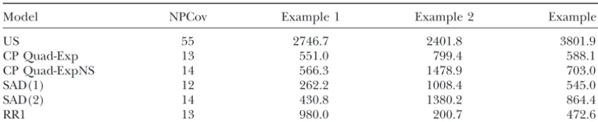
TABLE 1
Likelihood values for the simulated data sets based on unstructured covariance matrices
Model NPCov Example 1 Example 2 Example 3
US 55 2746.7 2401.8 3801.9
CP Quad-Exp 13 551.0 799.4 588.1
CP Quad-ExpNS 14 566.3 1478.9 703.0
SAD(1) 12 262.2 1008.4 545.0
SAD(2) 14 430.8 1380.2 864.4
RR1 13 980.0 200.7 472.6
US, unstructured covariance matrix; CP Quad-ExpNS, quadratic polynomial used to modelV(t), exponential function for⍀(t⫺s) with the nonstationary extension (Equation 6); RR1, linear random regression model with three additional parameters for the residual structure; NPCov, number of parameters in the covariance structure.
that the first-order bivariate structured antedependence V(t)⫽
冢
v2
1(t) v1(t)v2(t)12(t)
v1(t)v2(t)12(t) v22(t)
冣
. (10) model [SAD(1)] was well able to capture the covariance structures simulated under all these different assump-Variance functions can be modeled as for univariate charactertions (results not shown). The similarity between these process models with polynomial functions of time. For a
qua-dratic function, for instance,v2
1(t)⫽Var(g1(t))⫽exp(a1⫹ two approaches had already been pointed out in the b1t⫹c1t2) andv2
2(t)⫽Var(g2(t))⫽exp(a2⫹b2t⫹c2t2). univariate case for SAD(1) models and CP with an expo-Function12(t) represents the cross-correlation between the nential correlation function (Jaffre´zicet al.2003). On two traits at a given timet. A possible parametric modeling
the other hand, random regression models dealt poorly for this cross-correlation function is
with all the different covariance structures considered Corr(g1(t),g2(t))⫽ 12(t)⫽exp(⫺1t)⫺exp(⫺2t) (11) here, even when a cubic polynomial was used (involving
36 parameters for the covariance structure). for1,2⬎0. For practical purposes, it is interesting to note
that this correlation function is equal to 0 att⫽0, increases Simulations with unstructured covariance models:To to a maximum att⫽[ln(2/1)]/(2⫺ 1), and then decreases understand better the abilities and limitations of the to 0 at infinity.
different models, several patterns of covariance struc-A likelihood-ratio test can be used to examine specific
tures were investigated. To avoid favoring any of the hypotheses about the parameters. For example, testing if the
methodologies, data were simulated with unstructured cross-correlation between the two processes at all timestis
equal to zero is equivalent to testing if1⫽ 2. The cross- covariance matrices. A total of 2000 animals were consid-correlation function 12(t) can also be assumed constant: ered with five observations for each trait. As focus was 12(t)⫽r, which would imply that the cross-correlations are
on the cross-correlation modeling, quite simple struc-equal for allt.
tures for the variances and correlations of both variables
Estimation procedure:Parameters of these bivariate
charac-ter process models can be estimated with REML procedures, were chosen. Three examples are presented here. using, for example, the OWN function of ASREML (Gilmour In the first case, the data were generated using a
cross-et al.2002) as presented in appendix a. The nonstationary correlation that was stationary, symmetric, with quite parameterᐉ(Equation 6) is estimated at the same time as the
high values. With regard to the likelihood value (see other covariance parameters with standard REML procedures.
Table 1), a simple bivariate linear random regression The properties of the proposed bivariate covariance function
are studied inappendix b. model was found to be the most appropriate, followed
by the bivariate CP models and then the SAD models (all models had about the same number of parameters: EXAMPLE
from 12 to 14). Estimated cross-correlations obtained with the unstructured model and the bivariate linear
Simulation study:A simulation study was performed
random regresssion model are presented in Figure 1. to understand better the analogies between the
differ-In the second example, the cross-correlation was more ent methodologies: the bivariate CP model proposed
complex. Although the correlations between the traits here, the bivariate structured antedependence models
were still quite high, they were nonstationary and non-presented inJaffre´zic et al. (2003), and the random
symmetric. The bivariate quadratic random regression regression models. In a first set of simulations, data were
model did not converge and, on the other hand, the generated according to a bivariate CP model, with an
linear bivariate model was not able to deal adequately exponential “correlation” function (exp(⫺⌰(t ⫺ s)))
with this cross-correlation pattern. It was found for the and aV(t) structure defined aslnV(t)⫽A⫹Bt⫹Ct2.
character process model that the nonstationary exten-Different assumptions on parameters of⌰,A,B, andC
sion, using only one extra parameter (parameter ᐉ in were investigated, setting some elements to zero or
Figure1.—Estimated cross-correlations for example 1 of the simulation study for the unstructured model (US) and a bivariate linear random regression model (RR).
Table 1. The likelihood value was then higher than that early ages and then increasing and decreasing for late ages. The likelihood value was higher for SAD(2) than for the second-order SAD model with the same number
of parameters. Figure 2 gives the estimated cross-correla- for all the other models. It can be seen, however, in Figure 3, that this model was not able to adequately fit tions obtained with the unstructured model and with
the chosen bivariate CP model. the diagonal cross-correlation terms. On the other hand, although the likelihood value was a little lower than In the third example, the data were also generated
with nonsymmetric and nonstationary cross-correla- that with the second-order SAD model, the character process model was better able to capture the diagonal tions, with lower values than those for the first two
exam-ples. The diagonal cross-correlations were lower for cross-correlation pattern. These figures do show,
Figure 3.—Estimated cross-correlations for example 3 of the simulation study, with data simulated with an unstructured covariance matrix. [US, unstructured covariance matrix; CP, quadratic polynomial used to modelV(t), exponential function for ⍀(t⫺s) with the nonstationary extension (Equation 6); SAD, second-order bivariate structured antedependence model; RR, linear random regression model.]
ever, that even for the chosen models, there is still scope output were collected simultaneously from two replicate cohorts for each of 56 RI lines. Deaths were observed for improving the fit, although this might be difficult
while keeping the number of parameters reasonably low. every day, while egg counts were made every other day. For both mortality and reproduction, the data were
Empirical data—joint analysis of fecundity and
mor-tality in Drosophila:Age-specific measurements of re- pooled into 11 5-day intervals for analysis. Mortality rates were log transformed and reproductive measures were production and mortality rates were obtained from 56
different recombinant inbred (RI) lines ofD. melanogas- square-root transformed so that the age-specific mea-sures were approximately normally distributed.
ter, which are expected to exhibit genetically based
varia-tion in longevity and reproducvaria-tion ( J. W.Curtsinger Parameter estimates for the different methodologies were obtained with ASREML using the OWN function and A. A.Khazaeli, unpublished results). Age-specific
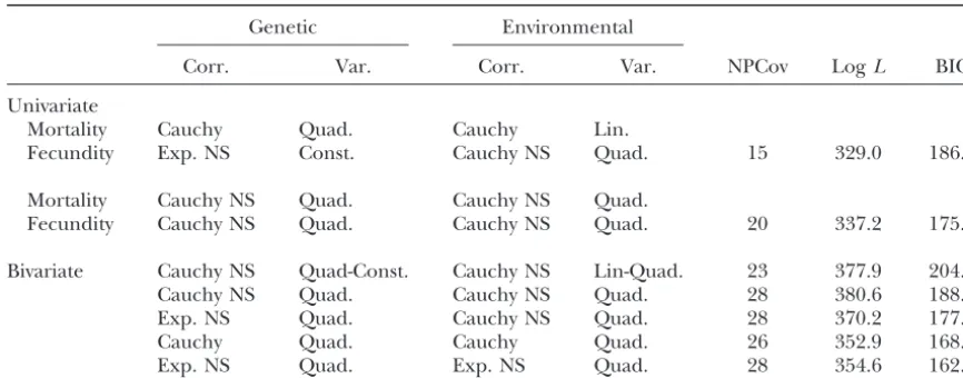
TABLE 2
Likelihood values and BIC criterion (Schwarz1978) for univariate and bivariate genetic analyses
of fecundity and mortality in Drosophila
Genetic Environmental
Corr. Var. Corr. Var. NPCov LogL BIC
Univariate
Mortality Cauchy Quad. Cauchy Lin.
Fecundity Exp. NS Const. Cauchy NS Quad. 15 329.0 186.7
Mortality Cauchy NS Quad. Cauchy NS Quad.
Fecundity Cauchy NS Quad. Cauchy NS Quad. 20 337.2 175.6
Bivariate Cauchy NS Quad-Const. Cauchy NS Lin-Quad. 23 377.9 204.8
Cauchy NS Quad. Cauchy NS Quad. 28 380.6 188.2
Exp. NS Quad. Cauchy NS Quad. 28 370.2 177.8
Cauchy Quad. Cauchy Quad. 26 352.9 168.2
Exp. NS Quad. Exp. NS Quad. 28 354.6 162.2
In both cases the logarithms of the variances were modeled, such as lnv2(t)⫽a⫹bt⫹c t2andln(V(t))⫽ A⫹Bt⫹Ct2withA,B, andC2⫻2 symmetric matrices. Corr., correlation; Var., variance; Quad., quadratic; Lin., linear; Exp., exponential; Const, constant.
BIC criterion (Schwarz1978;Jaffre´zicandPletcher in the methodology section). The main improvement of the bivariate model lies in its ability to model the 2000): BIC⫽lnL⫺ 0.5ncln(N⫺p), where lnLis the
REML likelihood value,ncis the number of covariance cross-covariance structure. The likelihood value of the bivariate model (Log L ⫽ 377.9) was indeed much parameters in the model,p is the number of fixed
ef-fects, and Nis the total number of observations. Stan- higher than that for the two univariate analyses (LogL⫽
329.0). Therefore, taking into account the correlation dard likelihood-ratio tests could be used for nested
mod-els. Specific cases include testing if certain parameters function between the two variables fits the actual process much better. Estimates obtained for the chosen bivari-in matricesV(t) or⌰are equal to zero. A nonparametric
mean function was used for both traits (i.e., a separate ate model are given in Table 3 and the first graph of Figure 4 gives the genetic cross-correlation estimates. mean was fitted for each distinct age in the data), which
ensures a consistent estimate of the covariance structure They were found to be negative at all ages, nonstationary and nonsymmetric. Fecundity and mortality were more (Diggleet al.1994).
The best models chosen in the univariate analyses are strongly negatively correlated at a similar age (diagonal terms), and the correlation intensity decreased when given in the first part of Table 2. For the genetic part,
a Cauchy correlation with quadratic variance was chosen ages became farther apart.
As they allow a simple and straightforward extension for mortality and a nonstationary exponential
correla-tion with a constant variance was chosen for fecundity. to the multivariate case, random regression models (RRM) are most often used for multivariate analyses of Many different correlation and variance functions were
investigated for the bivariate analysis and the best ones longitudinal data. They may not always, however, be the most appropriate methodology. In this example, for regarding the likelihood value and BIC criterion are
given in Table 2. In the bivariate model, the correlation instance, the likelihood value was much higher for the character process approach (Log L⫽ 377.9) than for function has to be the same for the two variables and
was chosen here to be a nonstationary Cauchy correla- a bivariate quadratic random regression model (Log
L⫽134.7), despite having far more parameters (42 for tion (with parameterᐉ of the nonstationary extension
as in Equation 6). For the variance function, more flex- the RRM compared to 23 for the CP model). Moreover, increasing the order of the polynomials dramatically ibility can be achieved in the choice of the function by
setting some parameters of matricesA,B, andCto zero. increases the number of parameters (for instance, from quadratic to cubic: 42 to 72 parameters).
In the bivariate model, the chosen function was, as in
the univariate case, quadratic for mortality and constant Although the difference was not as important as for random regression models, the likelihood value was also for fecundity. Estimates obtained for the variance and
correlation functions for fecundity and mortality were higher, in this example, for the bivariate CP model than for a bivariate structured antedependence model very similar with the univariate and bivariate models
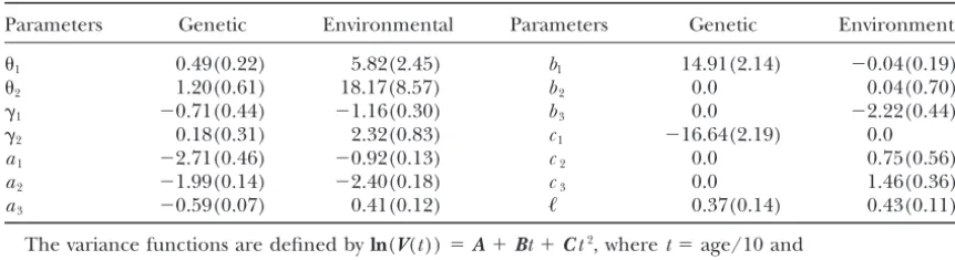
TABLE 3
Parameter estimates (and standard errors) for the bivariate genetic analysis of fecundity and mortality in Drosophila with the best-fitting bivariate character process model, for the BIC criterion, given in Table 2
Parameters Genetic Environmental Parameters Genetic Environmental
1 0.49(0.22) 5.82(2.45) b1 14.91(2.14) ⫺0.04(0.19)
2 1.20(0.61) 18.17(8.57) b2 0.0 0.04(0.70)
␥1 ⫺0.71(0.44) ⫺1.16(0.30) b3 0.0 ⫺2.22(0.44)
␥2 0.18(0.31) 2.32(0.83) c1 ⫺16.64(2.19) 0.0
a1 ⫺2.71(0.46) ⫺0.92(0.13) c2 0.0 0.75(0.56)
a2 ⫺1.99(0.14) ⫺2.40(0.18) c3 0.0 1.46(0.36)
a3 ⫺0.59(0.07) 0.41(0.12) ᐉ 0.37(0.14) 0.43(0.11)
The variance functions are defined byln(V(t))⫽A⫹Bt⫹Ct2, wheret⫽age/10 and
A⫽
冢
a1a3 a3a2冣
and similarly for matricesBandC. Parameters1,2,␥1, and␥2define matrix⌰as specified inappendix a for the Cauchy correlation function, andᐉis the nonstationary parameter (Equation 6).
The estimated genetic cross-correlations obtained estimated phenotypic cross-correlations and the un-structured estimates, the Vonesh concordance coeffi-with the three methodologies are presented in Figure
cient (Vonesh et al. 1996) was used, as presented by 4. Their patterns were found to be very different, even
Jaffre´zic and Pletcher (2000), considering the un-between the bivariate CP and SAD models, although
structured estimates as the correct values. there was only a small difference in their likelihood
The concordance coefficients were 0.77 for the CP values. As the true genetic cross-correlations are not
model, 0.52 for the SAD model, and 0.73 for the RR known, it is difficult, however, to know which pattern
model (a perfect fit being at 1.0). As shown with the is the closest to reality and how much discrepancy still
likelihood value, the bivariate character process model remains compared to the actual values.
fit best the phenotypic cross-correlation structure. On To address these issues, a phenotypic analysis was
the other hand, the goodness of fit was found higher performed on these data, which allows us to obtain
for the bivariate random regression model than for the estimates for an unstructured covariance matrix (22⫻
structured antedependence model (0.73 compared to 22). This was not possible in the genetic study due to
0.52), although the likelihood value was much higher the very large number of parameters to be estimated.
for the SAD model (Log L⫽ 183.8) than for the RR Estimated phenotypic cross-correlations obtained with
model (LogL⫽67.7). The SAD models were therefore the different models are presented in Figure 5 and the
in this case better able to model the covariance structure unstructured estimates were considered as the reference
for each trait separately, as in univariate analysis, model. Once again, the four estimated patterns were
whereas the random regression models were better able found to be very different. As in the genetic analysis,
to fit the cross-correlation structure. The choice of the the likelihood value was the highest for the character
model should therefore not be made regarding the process model (⫽ 197.1 with a nonstationary Cauchy
likelihood value only, but also depends on the priorities correlation function and quadraticV(t) function, with
of the study. In any case, in this particular study, the 14 parameters, BIC⫽ 58.6), compared to a bivariate
character process model was more appropriate than the SAD(1) model (Log L ⫽ 183.8, with 12 parameters,
other two methodologies. BIC⫽53.0), a bivariate SAD(2) model (LogL⫽185.9,
Figure 5 shows, however, that the obtained cross-cor-with 14 parameters, BIC⫽47.4), and a quadratic
bivari-relation patterns were still all quite different from the ate random regression model (LogL⫽67.7, 21
parame-unstructured phenotypic estimates and that there is still, ters, BIC⫽ ⫺97.7). The highest likelihood value,
ob-therefore, scope for improvement. tained here with the bivariate CP model, is still, however,
quite far away from that of the unstructured model (Log
L ⫽ 535.6). But as the number of parameters in the
DISCUSSION unstructured model is very large (⫽253), its BIC value
Figure4.—Estimated genetic cross-correlations between fecundity and mortality obtained with the chosen CP model, a bivariate SAD(1) model, and a quadratic random regression model.
els the covariance structure with a small number of properties of the univariate character process approach and simultaneously allow a parametric modeling of the interpretable parameters. A special case of these models
has been independently proposed in the statistical litera- cross-covariance structure. The proposed extension was based on an idea presented by Syet al.(1997) for the ture, namely the Ornstein-Uhlenbeck process (Taylor
et al.1994). It is equivalent to a character process model Ornstein-Uhlenbeck process and was generalized to
other kinds of correlation functions, including those with an exponential correlation function and constant
variances and represents a continuous time extension that are nonstationary.
Models were presented here in the bivariate case, but of a first-order autoregressive model.
We proposed an extension of the univariate character extension to the analysis of more than two correlated function-valued traits is straightforward and accom-process model to the multivariate case. Our goal was to
Figure5.—Estimated phenotypic cross-correlations between fecundity and mortality obtained with the unstructured model (US); a character process model CP Quad-CauchyNS: quadratic polynomial used to modelV(t), Cauchy function for⍀(t⫺s) with the nonstationary extension; a bivariate SAD(1) model; and a quadratic random regression model.
The first part of the simulation study highlighted the data and that the three models (random regression, structured antedependent, or character process) can similarities between the bivariate CP models with an
exponential correlation and bivariate first-order SAD be worthwhile depending on the particular biological phenomenon studied. When the cross-covariance struc-models (Jaffre´zicet al.2003), as in the univariate case.
Further differences between the two approaches appear ture is symmetric and stationary with quite high correla-tions, the most appropriate model to use might be a when higher orders of antedependence are considered
or when other parametric correlation functions are used simple random regression model. When the cross-corre-lation structure becomes more complex it should be in the CP models.
It was found in the second part of the simulation study either structured antedependence or character process models, especially because the number of parameters that the choice of the most appropriate methodology is
Sy, J. P., J. M. G. TaylorandW. G. Cumberland, 1997 A stochastic
dramatically increases. For the Drosophila analysis, the
model for the analysis of bivariate longitudinal AIDS data.
Biomet-bivariate character process model proved to be the most rics53:542–555.
Taylor, J. M. G, W. G. CumberlandandJ. P. Sy, 1994 A stochastic
appropriate.
model for analysis of longitudinal AIDS data. J. Am. Stat. Assoc.
The multivariate extension of the character process
89:727–736.
models represents a flexible and powerful technique Vonesh, E., V. ChinchilliandK. Pu, 1996 Goodness-of-fit in
gener-alized nonlinear mixed-effects models. Biometrics52:572–587.
for the genetic analysis of two or more function-valued
traits. Although the observed measurements are avail- Communicating editor: M. K.Uyenoyama able only on a discrete timescale, this approach can
model the fact that the underlying process is continuous
and therefore can deal with highly unbalanced data. As APPENDIX A: IMPLEMENTATION variance parameters are assumed to change with time,
As suggested bySyet al. (1997), to calculate the matrix other environmental factors of heterogeneity could be
exponentiation used in the correlation functions, diago-included in the variance modeling, as suggested by
nalization of matrix⌰is used, Foulley and Quaas (1995). Further research might
extend these multivariate models to include the genetic ⌰⫽ ⌫⌳⌫⫺1, (A1)
analysis of nonnormally distributed traits, as studied by
where⌳is a diagonal matrix of the distinct eigenvalues PletcherandJaffre´zic(2002) in the univariate case.
1and2of⌰, and⌫is a 2⫻2 matrix whose columns
We are most grateful to Jean-Louis Foulley, William G. Hill, Nancy
are the right eigenvectors. The matrix exponential is
Heckman, Jay Beder, and two anonymous referees for very interesting
then written and evaluated as
comments and ideas. Thanks go to J. Curtsinger and A. Khazaeli for generously providing published and unpublished data.
e⫺⌰(t⫺s)⫽⌫e⫺⌳(t⫺s)⌫⫺1. (A2) For the exponential correlation,
LITERATURE CITED
exp(⫺⌰(t⫺s))⫽
冢
␥1 ␥2 1 1冣冢
e⫺1(t⫺s) 0 0 e⫺2(t⫺s)
冣冢
1 ␥2 ␥1 1
冣
⫺1 , DeRisi, J. L., V. R. Iyer andP. O. Brown, 1997 Exploring the
metabolic and genetic control of gene expression on a genomic
scale. Science278:680–686. (A3)
Diggle, P. J., K. Y. LiangandS. L. Zeger, 1994 Analysis of
Longitudi-nal Data. Oxford University Press, Oxford. where parameters␥1and␥2are the elements of matrix
Foulley, J. L., andR. L. Quaas, 1995 Heterogeneous variances in ⌫
(Syet al.1997). The Gaussian is similar, with (t⫺s)
Gaussian linear mixed models. Genet. Sel. Evol.27:211–228.
being replaced by (t⫺s)2. For the Cauchy correlation, Gabriel, K. R., 1962 Ante-dependence analysis of an ordered set
of variables. Ann. Math. Stat.33:201–212. taking advantage of the fact that ⌰⫺1 ⫽ ⌫⌳⫺1⌫⫺1, it
Gilmour, A. R., B. J. Gogel, B. R. Cullis, S. J. WelhamandR.
follows that Thompson, 2002 ASREML User Guide Release 1.0. VSN
Interna-tional, Hemel Hempstead, UK.
Jaffre´zic, F., andS. D. Pletcher, 2000 Statistical models for esti- (I⫹⌰(t⫺s)2)⫺1⫽
冢
1 ␥2␥1 1
冣
mating the genetic basis of repeated measures and otherfunction-valued traits. Genetics156:913–922.
Jaffre´zic, F., I. M. S. White, R. ThompsonandP. M. Visscher, 2002 ⫻
冢
1/(1⫹ 1(t⫺s)2) 00 1/(1⫹ 2(t⫺s)2)
冣
Contrasting models for lactation curve analysis. J. Dairy Sci.84:968–975.
Jaffre´zic, F., R. ThompsonandW. G. Hill, 2003 Structured
antede-⫻
冢
1 ␥2␥1 1
冣
⫺1
.
pendence models for genetic analysis of multivariate repeated measures in quantitative traits. Genet. Res.82:55–65.
Meuwissen, T. H. E., andM. H. Pool, 2001 Autoregressive versus
For the variance functionsV(t), an eigenvalue
decom-random regression test-day models for prediction of milk yields.
position,lnV(t)⫽ P(t)⌬(t)Pⴕ(t), can also be used. It
Interbull Bull.27:172–178.
Meyer, K., 2001 Estimating genetic covariance functions assuming follows thatV(t)1/2⫽P(t)exp(1⁄
2⌬(t))P(t)⬘.
a parametric correlation structure for environmental effects. Parameter estimations were obtained using the OWN Genet. Sel. Evol.33:557–585.
function of ASREML (Gilmouret al. 2002), which re-Nunez-Anton, V., andD. L. Zimmerman, 2000 Modeling
non-sta-tionary longitudinal data. Biometrics56:699–705. quires us to provide the first derivatives of the covariance
Pletcher, S. D., andC. J. Geyer, 1999 The genetic analysis of age- matrix with respect to each parameter. The nonstation-dependent traits: modeling a character process. Genetics153:
ary parameterᐉof Equation 6 is obtained at the same
825–833.
Pletcher, S. D., andF. Jaffre´zic, 2002 Generalized character pro- time as the other parameters of the covariance matrix. cess models: estimating the genetic basis of traits that cannot be
observed and that change with age or environmental conditions. Biometrics58:157–162.
Pletcher, S. D., D. HouleandJ. W. Curtsinger, 1998 Age-specific
properties of spontaneous mutations affecting mortality inDro- APPENDIX B:
sophila melanogaster.Genetics148:287–303. PROPERTIES OF THE DEFINED BIVARIATE
Pletcher, S. D., S. J. Macdonald, R. Marguerie, U. Certa, S. C. CHARACTER PROCESS COVARIANCE FUNCTION Stearnset al., 2002 Genome-wide transcript profiles in aging
and calorically restrictedDrosophila melanogaster.Curr. Biol.12 WhenJ times of measurement are available for two
(9): 712–723.
variablesY1 andY2, and for each individuali, observa-Schwarz, G., 1978 Estimating the dimension of a model. Ann. Stat.
whole genetic covariance matrixGof dimension (2J⫻ nential function is considered. In this case, matrix⍀is defined as for the bivariate Ornstein-Uhlenbeck process 2J) can be written asG⫽V⍀Vⴕ. By construction
(Equa-tion 5), matrixG will be symmetric. MatrixVis block (Syet al. 1997) and therefore satisfies the positive defi-niteness property. When considering other functions as diagonal:V⫽(Vj)j⫽1,J, whereVjare 2 ⫻2 matrices
de-fined by Vj ⫽ (V(tj))1/2, where ln V(tj) ⫽ A ⫹ Btj ⫹ proposed in the univariate case byPletcherandGeyer
(1999), such as Gaussian or Cauchy, the property is
Ct2
j, or is specified as in Equation 10. In both cases,
matri-cesVj, forj⫽1, . . . , J, are positive definite. Matrix⍀ maintained. Therefore, the proposed function for the
bivariate CP model satisfies the theoretical require-is a 2J⫻2Jsymmetric matrix defined, for (i,j⫽1, . . . ,
J), by⍀(2(i⫺1)⫹1:2i, 2(j⫺1)⫹1:2j)⫽⍀ij, where ments of a covariance function as it is symmetric and