Selection in a Subdivided Population With Local Extinction and Recolonization
Joshua L. Cherry
1Department of Organismic and Evolutionary Biology, Harvard University, Cambridge, Massachusetts 02138
Manuscript received December 13, 2002 Accepted for publication March 4, 2003
ABSTRACT
In a subdivided population, local extinction and subsequent recolonization affect the fate of alleles. Of particular interest is the interaction of this force with natural selection. The effect of selection can be weakened by this additional source of stochastic change in allele frequency. The behavior of a selected allele in such a population is shown to be equivalent to that of an allele with a different selection coefficient in an unstructured population with a different size. This equivalence allows use of established results for panmictic populations to predict such quantities as fixation probabilities and mean times to fixation. The magnitude of the quantityNese, which determines fixation probability, is decreased by extinction and recolonization. Thus deleterious alleles are more likely to fix, and advantageous alleles less likely to do so, in the presence of extinction and recolonization. Computer simulations confirm that the theoretical predictions of both fixation probabilities and mean times to fixation are good approximations.
T
HE consequences of population subdivision for evol- tion of an infinite population size. These results provide ution depend on the nature of gene flow between not only fixation probabilities but also a complete de-subpopulations. Gene flow might be restricted to ordi- scription of the trajectory of the frequency of a selected nary migration, but might also include extinction of allele. This description is equivalent to that of an un-subpopulations followed by recolonization. Extinction structured population with a different size and a differ-and recolonization affect not only the amount of neutral ent selection coefficient.variation maintained in the population, but also the effi-cacy of natural selection compared to stochastic change in allele frequency.
MODEL AND RESULTS In the absence of extinction and recolonization,
sub-division increases the effective population size. None- To obtain results for a finite island model of subdivi-theless, fixation probabilities of alleles subject to genic sion, I first consider a model with a single sink popula-selection are unaffected by subdivision under fairly gen- tion and a source population with constant allele fre-eral conditions (Maruyama 1970, 1974). These facts quency. The results translate to a quasi-equilibrium for can in some cases be reconciled with the aid of the subpopulations in a finite island model.
notion of effective selection coefficient (se;Cherryand Consider a haploid population that receives migrants
Wakeley2003). from a source population and is also subject to
extinc-Extinction and recolonization lower effective popula- tion and subsequent recolonization by a single individ-tion size (Slatkin1977;MaruyamaandKimura1980; ual from that source population. Suppose that a locus
WhitlockandBarton1997). When sufficiently strong has two allelic forms, a and A, and that there is no
they can reduce effective size below the actual popula- further mutation. Denote byxthe frequency of theA tion size. Extinction and recolonization can affect the allele in the sink population, and letxbe its (constant) probability of fixation of alleles subject to selection frequency in the source population. Letmbe the rate
(Barton1993). of migration and letbe the probability of extinction
Barton(1993) has derived expressions for the fixa- and recolonization in any generation. Assume for the
tion probability of a favored allele initially present in a moment that there is no selection. single copy in an infinite population with extinction
If there were no extinction and recolonization, the and recolonization. Here I present results that cover
equilibrium distribution of the allele frequencyxwould deleterious as well as advantageous alleles, apply to any
be well approximated by a-distribution (Wright1931). initial allele frequency, and do not require the
assump-This follows from a diffusion approximation. The case with extinction and recolonization may not be amenable to a diffusion approach because
extinction/recoloniza-1Address for correspondence:National Center for Biotechnology
Infor-tion events drastically change the allele frequency in the mation, National Library of Medicine, National Institutes of Health,
course of a generation. However, we need not be con-8600 Rockville Pike, Bldg. 45, Bethesda, MD 20894.
E-mail: [email protected] cerned with the exact distribution for the present
poses. Because we are interested only in the mean and 1⫺FST⫽ (N⫺1)(2m⫺m2)
N⫺(N⫺1)(1⫺m)2
冢
1⫺
1⫺(1⫺ )(1⫺1/N)(1⫺m)2
冣
variance of the change in allele frequency in agenera-tion, the main concern is to find the expected value of
⬇ 2Nm
2Nm⫹N ⫹1, x(1⫺x), which is half the expected heterozygosity. The
mean change in allele frequency due to selection is
where the approximate equality holds for smallm, large approximately proportional to this quantity. The
com-N, and small. The first factor in the exact form would ponent of the variance of this change that is due to
give 1⫺FSTif there were no extinction and
recoloniza-ordinary drift is also approximately proportional to this
tion and is approximately equal to 2Nm/(2Nm ⫹1), a quantity. The additional variance due to extinction/
familiar approximation for 1⫺FSTfor an island model
recolonization events can be calculated separately and
with ordinary migration (Wright 1940; Dobzhansky combined with this.
and Wright1941). The second factor represents the
It is convenient to think in terms of the “virtual
hetero-additional loss of heterozygosity due to extinction/re-zygosity”H, the expected value of 2x(1⫺x). This
quan-colonization events; for ⫽ 0 it equals one, and it is tity can be interpreted as the probability that two copies
less than one for ⬎ 0. The approximate equality is of the locus, drawn uniformly and independently from
equivalent to a case of the expression forFST given by
the population with replacement, are in different allelic
WhitlockandBarton(1997, Equation 21), with their
states. We can write a recursion forHthat depends on
k equal to 1⁄
2. This approximation makes it clear that
the mean allele frequency. For the two copies of the
extinction and recolonization decreases heterozygosity gene to be in different allelic states, it is necessary that
and that the expression for 1 ⫺ FST is close to 2Nm/
there has not just been an extinction/recolonization
(2Nm⫹1) when ⫽0. Note that 1⫺FSTis independent
event (probability 1⫺ ) and also that the same copy
ofx, which might not have been obvious from the start. of the locus has not been sampled twice (probability
The sink population described above serves as a 1 ⫺ 1/N). If these criteria are met there are three
model for a subpopulation in a finite island model. In possibilities to consider. If neither sampled allele is a
this model D demes (“islands”), each consisting of N
migrant, the probability that the alleles are different is
individuals, exchange migrants among themselves and simply the value of H in the previous generation. If also serve as sources for recolonization. Letxnow refer exactly one is a migrant, the probability depends on the to the frequency of theAallele in the population as a value of E[x] in the previous generation and is equal whole (the mean of the within-deme allele frequencies). toE[x](1⫺x)⫹ (1⫺E[x])x.If both are migrants, this In any generation, the population as a whole in effect probability is that of picking two different alleles from serves as a source population for any particular deme, the source population, 2x(1 ⫺x). Putting this all to- with an allele frequency x. In the finite island model,
gether gives in contrast to the source-sink model, the value of x
changes over time. However, when the number of
Ht⫹1⫽(1⫺ )(1⫺1/N)
demes is large,xchanges only slowly compared to the rate of equilibration of within-deme allele frequencies, ⫻[(1⫺m)2Ht⫹2m(1⫺m)(E[x](1⫺x)⫹(1⫺E[x])x)
unless selection is very strong (see below), and so a
⫹m22x(1⫺x)] , (1)
quasi-equilibrium is attained (Wright1931; Dobzhan-skyandWright1941). This is so because the stochastic whereHtis the heterozygosity at timetandE[x] refers
change in the population as a whole is the mean of to the expectation in the previous generation. At
equi-theDindependent within-deme stochastic changes. The librium E[x]⫽ x. The equilibrium condition for H is
quasi-equilibrium distribution of within-deme allele fre-therefore
quency approaches the equilibrium distribution that holds for the sink population of a source-sink model.
H⫽(1⫺ )(1⫺1/N)[(1⫺m)2H⫹(2m⫺m2)2x(1⫺x)] .
Thus FST, the fractional loss of heterozygosity due to
(2)
subdivision, is given approximately by Equation 4. This
Solution forHgives expression will allow derivation of a diffusion
approxi-mation for the behavior of an allele in the population
H⫽ (1⫺ )(1⫺1/N)(2m⫺m
2)
1⫺(1⫺ )(1⫺1/N)(1⫺m)22x(1⫺x) as a whole when the number of demes is large. The above treatment of the quasi-equilibrium ne-⫽ (N⫺1)(2m⫺m2)
N⫺(N⫺1)(1⫺m)2
冢
1⫺
1⫺(1⫺ )(1⫺1/N)(1⫺m)2
冣
2x(1⫺x) . glected selection. Selection raises two issues. First, if selection is very strong,xmay change so rapidly that a (3)quasi-equilibrium is not approached. Second, selection The quantityFST, which is later interpreted as the frac- will alter the (quasi-) equilibrium distribution of allele
tional loss of heterozygosity due to subdivision, is de- frequency, even in the source-sink model, where a true fined by 1⫺ FST⬅ E[x(1 ⫺x)]/x(1⫺x)⫽H/2x(1⫺ equilibrium is reached. If selection is weak compared
to stochastic change in allele frequency within a
ulation, it has negligible effect on the (quasi-) equilib- components, one corresponding to binomial sampling and another corresponding to extinction and recoloni-rium distribution of allele frequency. The mean change
due to selection is proportional tos, and the variance zation. Conditional on no extinction, the second moment aboutE[x⬘] is (1/N)E[x⬘](1⫺E[x⬘]) orⵑ(1/N)x(1⫺ due to ordinary drift is proportional to 1/N. Thus a
sufficient condition for directional change to be weaker x). Conditional on extinction and recolonization,x⬘is 1 with probabilityxand 0 with probability 1⫺x,so the than stochastic change within a deme is
second moment about E[x⬘] is x(1⫺E[x⬘])2⫹ (1⫺
|Ns|Ⰶ1 , (5)
x)E[x⬘]2⬇x(1⫺ x)2⫹(1⫺x)x2. Thus the variance in x⬘as a function ofxis given by
which is conservative because it does not take into ac-count the stochastic change due to extinction and
recol-Var(x⬘)⬇(1⫺ )1
Nx(1⫺x)⫹ [x(1⫺x)
2⫹(1⫺x)x2] .
onization. This condition also guarantees that the rate
of change ofxis small enough that a quasi-equilibrium (7)
is approached. The per-generation change inxdue to
Because 1⫺ ⬇ 1, this simplifies to selection is at most aboutsx(1⫺x) (this would be the
change if all demes had the same allele frequency). The
Var(x⬘)⬇1
Nx(1⫺x)⫹ [x(1⫺x)
2⫹(1⫺x)x2] . (8)
maximum value of this change is therefore s/4. As is evident from Equation 1, heterozygosity in a deme
de-The expected value of this expression follows readily cays toward its equilibrium on a timescale ofN
genera-from our expressions forE[x] andE[x(1⫺x)]. Using tions or faster (migration and
extinction/recoloniza-E[x]⫽xandE[x(1⫺ x)]⫽(1⫺ FST)x(1⫺ x), we
ob-tion hasten this decay). Thus condiob-tion (5) is also
tain sufficient for the quasi-equilibrium to be approached.
Because stochastic change in the whole population is a E[Var(⌬x)]⫽E[Var(x⬘)] much weaker force than stochastic change in a
subpopu-lation, selection may be sufficiently weak in the sense ⬇
冦
1N(1⫺FST)⫹ [2⫺(1⫺FST)]
冧
x(1⫺x) .that |Ns| Ⰶ 1 and yet strongly affect the trajectory of
(9) allele frequency in the population as a whole. I assume
that this condition holds in all that follows. ThereforeV
⌬x,the variance in the change in population-Let xi be the allele frequency in theith deme. The wide allele frequencyx, is given by
mean change in allele frequency in this deme due to selection isⵑsxi(1⫺ xi) in one generation. The mean V
⌬x⫽ 1
D2
兺
iVar(⌬xi) in the entire population is the mean of thesxi(1 ⫺xi)
over alli, orⵑsE[xi(1 ⫺xi)]⫽ (1⫺FST)sx(1 ⫺x). This
⬇1
DE[Var(⌬xi)]
mean has the same form as that in a panmictic popula-tion, but withsreplaced by (1⫺FST)s. Thus the effective
selection coefficientseis given by ⬇1
D
冦
1
N(1⫺FST)⫹ [2⫺(1⫺FST)]
冧
x(1⫺x) . (10) se⫽(1⫺FST)sThis variance is proportional tox(1⫺x), as it is in a ⫽ (N⫺1)(2m⫺m2)
N⫺(N⫺1)(1⫺m)2
冢
1⫺
1⫺(1⫺ )(1⫺1/N)(1⫺m)2
冣
s panmictic population. The definition of variance effec-tive population size is given by V⌬x⫽(1/Ne)x(1⫺x).Therefore
⬇ 2Nm
2Nm⫹N ⫹1s. (6)
Ne⬇
ND
(1⫺ FST)⫹N[2⫺ (1⫺FST)]
, (11)
An analogous treatment of the variance in ⌬x will yield the effective population size Ne. This variance is
approximated by a simple function of the expected vari- withFSTgiven by Equation 4.Necan be larger or smaller
than the actual population sizeND, depending on the ance of within-deme change in allele frequency. To
obtain this quantity I first derive an expression for this parametersN,m, and.
These results show that a selected allele in a subdi-variance conditional on within-deme allele frequency
and then take the mean across the quasi-equilibrium vided population with extinction and recolonization be-haves much like an allele with a different selection coef-distribution of allele frequency.
Suppose thatxis the allele frequency within a deme ficient in a panmictic population with a different size. This follows from the fact that both the mean and the in one generation andx⬘is the frequency in the next.
The variance of ⌬x, the change in allele frequency, is variance of the change in allele frequency are approxi-mately proportional tox(1⫺ x), as they are in a panmic-equal to the variance ofx⬘, the second moment of x⬘
about E[x⬘]. Because the mean change in allele fre- tic population (expressions for this mean and variance completely determine the diffusion approximation). quency in a single generation is small fors, m, Ⰶ1,
seandNe, are given by Equations 6 and 11. In the pres- Predictions of fixation probabilities and fixation times
follow from a combination of the theory presented here ence of extinction and recolonization, the value ofNese,
which determines fixation probability, is different from with classical diffusion results. Substitution ofNeandse
forNandsin a familiar expression for fixation probabil-its value in a panmictic population. The magnitude of
this product is decreased by extinction and recoloniza- ity (Wright1931) gives this probability as tion. Specifically,
1⫺e⫺2Nesex0 1⫺e⫺2Nese , Nese⬇
(1⫺FST)
(1⫺ FST)⫹N[2 ⫺(1⫺ FST)]
NDs. (12)
wherex0is the initial allele frequency in the population
andseandNeare given by Equations 6 and 11. Similarly,
use of an expression given byKimuraandOhta(1969,
COMPUTER SIMULATIONS Equation 17), withs
esubstituted forsand adjustments
made for haploidy, gives predictions of mean times to To test the approximations used above, I ran
com-fixation. puter simulations and compared the results to
theoreti-Tables 1 and 2 compare such theoretical predictions cal predictions. In these simulations the state of the
to simulation results for s⫽ 10⫺3,N ⫽ 100, D⫽ 100,
population is represented by an array of D integers,
and various values ofmand. Table 1 shows predicted each corresponding to a deme. Each integer indicates
and observed probabilities of fixation of an allele ini-the number of copies of alleleAin the deme and hence
tially present as a single copy, relative to the neutral ranges from 0 toN. Each generation the new value for
fixation probability. All of the predictions are close to each deme is determined as follows. With probability
the observed quantities (largest deviation is 7%). Table the deme undergoes extinction and recolonization,
2 shows predicted and observed mean times to fixation. after which the new number ofAalleles isNwith
proba-The predictions are very close to the observations, dif-bility xand 0 with probability 1⫺x. With probability
fering by at most 2%. Simulations withs⫽3⫻10⫺4or
1⫺ the deme does not go extinct and the new number
s⫽ 10⫺4also demonstrate a good agreement between
is chosen from a binomial distribution. The index
pa-prediction and observation (data not shown). rameternof this binomial (number of “trials”) is equal
Tables 3 and 4 show relative fixation probabilities for toN. The probability parameterp(probability of
“suc-selectively disfavored alleles. Table 3 gives results fors⫽
cess”) is determined by the current allele frequency in
⫺3 ⫻ 10⫺4. The predictions are all very close to the
the demexi, the population-wide mean allele frequency
observations (within 3%). Table 4 shows results for a
x, the migration ratem, and the selection coefficients.
more strongly disfavored allele (s⫽ ⫺10⫺3), for which
Let p˜ ⫽(1⫺ m)xi⫹ mx.This would be the expected
fixation probabilities would be minuscule without ex-allele frequency in theith deme in the next generation
tinction and recolonization. For some sets of parame-if there were no selection. Therefore p ⫽ (1 ⫹ s)p˜/
ters, no fixations were observed in the simulations. This (1⫹sp˜).
is consistent with the very low predicted values of fixa-Figure 1 compares the distribution of allele
frequen-tion probability. For the other cases, the agreement cies among many independent simulation runs to
theo-between theory and observation is good (maximum de-retical predictions at two time points. In the simulations
viation is 15%). Without extinction and recolonization,
N⫽100,D⫽100,s⫽3⫻10⫺4,m⫽0.001, ⫽0.001,
or without population structure altogether, the relative and the initial allele frequency was 1/2 (each deme
fixation probability would be 4⫻10⫺8. Thus the theory
initially contained 50 Aand 50a alleles). The
predic-captures the more than seven orders of magnitude tions shown were obtained by iteration of the transition
change in fixation probability due to extinction and matrix for a Wright-Fisher population of 100 individuals.
recolonization. Predictions of fixation times are also The selection coefficient for this population was chosen
good for both values of selection coefficient (maximum such that the product of the population size and the
deviation 3%), as are predictions for s⫽ ⫺10⫺4 (data
selection coefficient was equal to Nese, with Ne and se
not shown). given by Equations 6 and 11. Time was scaled to account
Tables 5 and 6 show results for a smaller number of for the difference in effective size between the small
demes (D⫽ 30). Even with so few demes, predictions Wright-Fisher population and the subdivided
popula-of fixation probabilities are close to the simulation re-tion: the number of generations in the Wright-Fisher
sults (all within 6%). Fixation times (not shown) are population was smaller than that in the simulations by
also in excellent agreement with predictions. a factor of Ne/100. The plots demonstrate excellent
agreement between the predictions and the simulation results, confirming that the trajectory of allele frequency
DISCUSSION in the structured population is similar to that in a
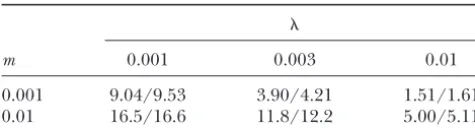
TABLE 3 TABLE 1
Predicted and observed relative fixation probabilities for Predicted and observed relative fixation probabilities for
s⫽ ⫺3⫻10⫺4,D⫽100, andN⫽100
s⫽10⫺3,D⫽100, andN⫽100
m 0.001 0.003 0.01 m 0.001 0.003 0.01
0.001 0.193/0.181 0.535/0.532 0.872/0.858
0.001 9.04/9.53 3.90/4.21 1.51/1.61
0.01 16.5/16.6 11.8/12.2 5.00/5.11 0.01 0.0352/0.0363 0.106/0.105 0.434/0.427
Fixation probabilities are given relative to that of a Fixation probabilities are given relative to that of a
selec-tively neutral allele for various values of migration rate (m) tively neutral allele. Numbers to the left of slashes are theoreti-cal predictions, and numbers to the right are observed values. and extinction probability (). Numbers to the left of slashes
are theoretical predictions, and numbers to the right are ob- In all cases the allele was initially present in a single copy. served values (simulation results). In all cases the allele was
initially present in a single copy.
ton(1993) for a favored allele in an infinite population, but applies much more generally.
Computer simulations confirm that these theoretical here describe the trajectory of the frequency of an allele
results make good predictions. Fixation probabilities under selection in the presence of this force when the
observed in simulations are close to theoretical predic-number of demes is large and a deme is recolonized by
tions. Predicted mean times to fixation also agree well a single haploid individual. The behavior of the
subdi-with simulation results. vided population was shown to be equivalent to that of a
The results presented here are based on the assump-certain panmictic population. The size of this equivalent
tion that an empty deme is recolonized by a single hap-panmictic population (Ne) is different from the actual
loid founder. Results can be quite different when recolo-size of the subdivided population. Ne can be larger or
nization involves more than one founding allele. For smaller than this actual size. The selection coefficient
example,FSTis raised by extinction and recolonization
in the equivalent panmictic population (se) is different
with just one founding allele, but can be lowered by from the actual selection coefficient.seis always smaller
extinction and recolonization when there are multiple in magnitude than the actual selection coefficient and
founders (Takahata 1994; Whitlock and Barton
has the same sign. Expressions forse andNe are given
1997). Thus with multiple founders |se| can be raised
by Equations 6 and 11. These allow application of
estab-rather than lowered by extinction and recolonization, lished results for panmictic populations to subdivided
although |se| can never be larger than |s|.
populations with extinction and recolonization.
Barton (1993) noted an apparent discrepancy
be-The productNesedetermines the probability of fixation
tween the Ne that applies to fixation probabilities of
of an allele. Extinction and recolonization reduces the
selected alleles and Nethat is relevant to maintenance
magnitude of this quantity. Thus selection plays less of a
of neutral variation. However, the value ofNegiven for
role in determining the fate of an allele in the presence
fixation probabilities was based on the assumption that of extinction and recolonization. This reflects the fact that
fixation probability depends onNes. The distinction
be-extinction and recolonization are additional stochastic
tweensandse, and hence betweenNesandNese, resolves
forces that can overwhelm the directional effects of selec-tion. This result is consistent with those obtained by
Bar-TABLE 4
Predicted and observed relative fixation probabilities for TABLE 2
s⫽ ⫺10⫺3,D⫽100, andN⫽100 Predicted and observed fixation times fors⫽10⫺3,
D⫽100, andN⫽100
m 0.001 0.003 0.01
0.001 1.07⫻10⫺3/ 0.0859/0.0763 0.618/0.582
m 0.001 0.003 0.01
0.97⫻10⫺3
0.001 34,798/34,106 24,513/24,367 9,894/9,813 0.01 1.11⫻10⫺6/0 8.76⫻10⫺5/0 0.0350/0.0304 0.01 10,337/10,178 9,804/9,729 7,820/7,837
Fixation probabilities are given relative to that of a selec-tively neutral allele. Numbers to the left of slashes are theoreti-Numbers to the left of slashes are theoretical predictions, and
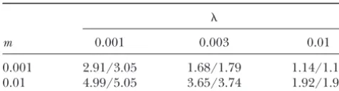
TABLE 6 TABLE 5
Predicted and observed relative fixation probabilities for Predicted and observed relative fixation probabilities for
s⫽ ⫺10⫺3,D⫽30, andN⫽100
s⫽10⫺3,D⫽30, andN⫽100
m 0.001 0.003 0.01 m 0.001 0.003 0.01
0.001 0.193/0.183 0.535/0.507 0.872/0.824
0.001 2.91/3.05 1.68/1.79 1.14/1.19
0.01 4.99/5.05 3.65/3.74 1.92/1.98 0.01 0.0352/0.0355 0.106/0.101 0.434/0.419
Fixation probabilities are given relative to that of a Fixation probabilities are given relative to that of a
selec-tively neutral allele. Numbers to the left of slashes are theoreti- tively neutral allele. Numbers to the left of slashes are theoreti-cal predictions, and numbers to the right are observed values. cal predictions, and numbers to the right are observed values.
In all cases the allele was initially present in a single copy. In all cases the allele was initially present in a single copy.
the apparent discrepancy: the ratio ofsetosis 1⫺FST, I thank Christina Muirhead and Jon Wilkins for comments on the
which approximately equals the ratio of the two values manuscript. This work was supported by National Science Foundation grant DEB-9815367 to John Wakeley.
ofNe given byBarton(1993) for the model analyzed
here. Thus the concept of effective selection coefficient allows the use of a single value ofNe to describe both
LITERATURE CITED the behavior of neutral variation and the probability of
fixation of an allele under selection. Barton, N. H., 1993 The probability of fixation of a favoured allele in a subdivided population. Genet. Res.62:149–157.
The results presented here have implications for the
Bulmer, M., 1991 The selection-mutation-drift theory of synony-interpretation of population-genetic data. Attempts mous codon usage. Genetics129:897–907.
have been made to estimate selection coefficients from Cherry, J. L., andJ. Wakeley, 2003 A diffusion approximation for selection and drift in a subdivided population. Genetics 163:
molecular data. For example, Bulmer (1991) and
421–428.
Hartl et al. (1994) estimated the selective cost of a Dobzhansky, T., andS. Wright, 1941 Genetics of natural popula-nonoptimal codon inEscherichia colias on the order of tions. V. Relations between mutation rate and accumulation of lethals in populations of Drosophila pseudoobscura. Genetics26:
10⫺9–10⫺8. What such studies actually estimate is the
23–51.
effective selection coefficientse. This quantity is of inter- Hartl, D. L., E. N. MoriyamaandS. A. Sawyer, 1994 Selection
est because it dictates the population-genetic behavior intensity for codon bias. Genetics138:227–234.
Kimura, M., andT. Ohta, 1969 The average number of generations of, in this example, alleles differing by synonymous
until fixation of a mutant gene in a finite population. Genetics changes. However, if one is interested in the physiology 61:763–771.
of bacteria and the magnitude of the decrease in growth Maruyama, T., 1970 On the fixation probability of mutant genes in a subdivided population. Genet. Res.15:221–225.
rate due to nonoptimal codons, the quantity of interest
Maruyama, T., 1974 A simple proof that certain quantities are inde-iss. Just as Necan differ by orders of magnitude from pendent of the geographical structure of population. Theor.
the actual population size,semight be radically different Popul. Biol.5:148–154.
Maruyama, T., andM. Kimura, 1980 Genetic variability and effec-froms. The difference between seandsmight explain
tive population size when local extinction and recolonization the discrepancy noted byBulmer(1991) between esti- of subpopulations are frequent. Proc. Natl. Acad. Sci. USA77: mates of “selection coefficients” and predictions based 6710–6714.
Slatkin, M., 1977 Gene flow and genetic drift in a species subject on physiological considerations.
to frequent local extinctions. Theor. Popul. Biol.12:253–262. Knowledge of the actual population size could be Takahata, N., 1994 Repeated failures that led to the eventual suc-used to obtain estimates ofsif there were no extinction cess in human evolution. Mol. Biol. Evol.11:803–805.
Whitlock, M. C., andN. H. Barton, 1997 The effective size of a and recolonization, sinceNeseis unaffected by that type
subdivided population. Genetics146:427–441.
of population structure. In the presence of extinction Wright, S., 1931 Evolution in Mendelian populations. Genetics16: and recolonization the actual population size is of no 97–159.
Wright, S., 1940 Breeding structure of populations in relation to help, since Nese is in this case altered by population
speciation. Am. Nat.74:232–248. structure. However, knowledge ofFSTcould be used to