Performance of Microcalcification Detection Algorithms

Abstract

SRIVASTAVA, VAIBHAV. Performance of microcalcification detection algorithms. (Under the direction of Dr Wesley Snyder)

Breast cancer is the most common malignancy in women and is three times more common than all gyneco-logic malignancies put together. The incidence of breast cancer has been increasing steadily from an incidence of 1:20 in 1960 to 1:8 women today. Seventy percent of all breast cancers are found through breast self-exams. However not all lumps are detectable by touch and mammography is a low-dose X-ray examination that can detect breast cancer up to two years before it is large enough to be felt. Some patterns of microcalcifications (small white deposits of calcium) give an early indication of cancer. Their small size makes their detection difficult for the radiologist. This brings in the role of CAD (Computer Aided Diagnosis) which serve as an assistant to the radiologist. In this thesis we have investigated the performance of three state of the art CAD techniques for the detection of microcalcifications in mammograms.

First, is a wavelet based technique which applies an adaptive wavelet filter to the input mammogram. Then it calculates HOS (Higher Order Statistics) values for maxima locations that are determined from the input image by an empirical method. This is followed by determination of a threshold using a cross entropy based thresholding algorithm. The thresholded image gives the locations of microcalcifications.

Second, is a technique that pre-processes the input mammogram with a tophat morphological filter which only preserves objects that are smaller than the size of the filter used in pre-processing. This is again followed by the determination of a threshold using the same thresholding algorithm as in the first technique. The thresholded image indicates the positions of microcalcifications. We have also done an investigation of co-occurrence matrix based entropy thresholding schemes. We found that two dimensional matrix based algorithms perform better than three dimensional based algorithms. Although both fail in case of images with high dynamic range which make them unsuitable for medical imaging. However the cross entropy based method performed better than co-occurrence matrix based techniques for both low as well as high resolution images.

PERFORMANCE OF MICROCALCIFICATION

DETECTION ALGORITHMS

by

Vaibhav Srivastava

A thesis submitted to the Graduate Faculty of

Department of Electrical and Computer Engineering

in partial satisfaction of the

requirements for the Degree of

Master of Science in Electrical Engineering

Department of Electrical And Computer Engineering

Raleigh

2005

Approved by:

__________________

Dr Wesley Snyder

Chair of Advisory Committee

__________________

__________________

Dr Edward Grant

Dr David Lalush

__________________

Biography

Acknowledgement

In the first place I would like to thank my father, Sri Satish Chandra Srivastava, my mother Srimati Anita and sister Disha Srivastava for their constant encouragement and values that allowed me to choose this career path. Next I would like to thank my adviser Dr Wesley Snyder for his most able and compassionate guidance. It was his constant encouragement and support that enabled me to complete this work. His guidance allied with most affable personality makes it a dream to work with him. I would also like to thank the imaging group at North Carolina State University headed by Dr Wesley Snyder for their help most notably, Karthik Krish, Geoff Chang and Pedro Lee. I would also like to thank North Carolina State University administration for its excellent institutional support throughout my studies.

Contents

List of Figures vi

List of Tables viii

1 Introduction 1

1.1 What are micro-calcifications . . . 2

1.1.1 Types of calcifications . . . 3

1.2 Selection of algorithms for comparison . . . 4

1.3 Synthesis of calcifications on mammograms . . . 5

1.3.1 Organization of the thesis . . . 6

2 Adaptive Wavelet Filtering 9 2.1 Wavelet based representation of images . . . 10

2.1.1 Normal subband decomposition . . . 10

2.1.2 Adaptive subband decomposition . . . 11

2.1.3 HOS test . . . 12

2.1.4 Algorithm . . . 13

2.1.5 Experimental results . . . 14

3 Entropy thresholding 18 3.1 Algorithms . . . 20

3.1.1 Minimum cross entropy thresholding . . . 20

3.1.2 Two dimensional co-occurrence matrix based . . . 21

3.1.3 Three dimensional co-occurrence matrix based . . . 24

4 Support Vector Machines 34

4.1 Review of support vector machine classifiers . . . 37

4.1.1 Linear SVMs . . . 37

4.1.2 Nonlinear support vector machines . . . 38

4.2 Successive enhancement learning algorithm . . . 40

4.3 Experiments . . . 41

4.3.1 Training phase . . . 41

4.3.2 Testing phase . . . 42

5 Conclusion 48

List of Figures

1.1 Typical mammogram . . . 2

1.2 Calcifications in the breast . . . 3

1.3 Low pass filter used in synthesis of microcalcifications . . . 6

1.4 Simulation of microcalcifications on normal mammogram region 1 . . . 7

1.5 Simulation of microcalcifications on normal mammograms region 2 . . . 8

2.1 Two dimensional subband decomposition using wavelet filters . . . 11

2.2 Adaptive subband decomposition structure . . . 12

2.3 8 search directions around the center pixel . . . 13

2.4 Best output with wavelet based approach. False positives = 1, False negatives = 1 (blue - true MC, red - detected MC) . . . 16

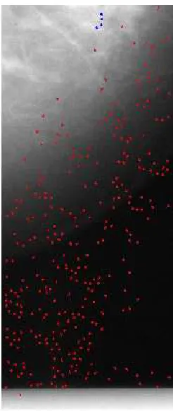
2.5 Worst output with wavelet based approach. False positives = 285, False negatives = 6 (blue -true MC, red - detected MC) . . . 17

3.1 Quadrants of co-occurrence matrix . . . 22

3.2 Input image for comparison of thresholding algorithms . . . 27

3.3 Thresholding the image in Figure 3.2 using algorithms in [41] . . . 28

3.4 Thresholding the image in Figure 3.2 using algorithms in [41] . . . 28

3.5 Thresholding the image in Figure 3.2 with scaling between 0-255 . . . 29

3.6 Thresholding the image in Figure 3.2 without scaling . . . 29

3.7 Output with cross entropy based approach for image which gave worst performance with the wavelet approach. False positives = 3, False negatives = 4 (blue - true MC, red - detected MC) 30 3.8 Output when cross entropy based thresholding does not work well. False positives = 8, False negatives = 41(blue - true MC, red - detected MC) . . . 31

4.1 Linear support vector classifier with separable data. Support vectors are circled. (From [7]) . . 36

4.2 Linear support vector classifier with non-separable data. Support vectors are circled. (From [7]) 38 4.3 Effect of high pass filtering (length = 41, cut off frequency = 0.125) on mammogram . . . 41

4.4 Selection of positive samples from the neighbourhood of a MC. Center pixel is shown black and extra positive locations selected are shown as gray . . . 42

4.5 Variation of error with the number of iterations for SEL algorithm . . . 43

4.6 Overall ROC curve with real microcalcifications . . . 44

4.7 Overall ROC curve with simulated microcalcifications . . . 45

List of Tables

2.1 Results with Wavelet based approach for varying µ and pre-threshold0t0 . . . 15

2.2 Results obtained for wavelet based algorithm with simulated microcalcifications . . . 15

3.1 Results with cross entropy based approach with variation of pre-threshold0t0 . . . 27

3.2 Results obtained for cross entropy based algorithm with simulated microcalcifications . . . 33

4.1 Results obtained with SVM classifier on training set, test set . . . 43

4.2 Overall results obtained with SVM classifier . . . 47

Chapter 1

Introduction

Breast cancer is the most frequent neoplasm in women in western countries and is the leading cause of cancer deaths among women age forty to forty-nine. It is second only to lung cancer as a cause of cancer death among women. Breast cancer accounts for one of every three cancer diagnoses in women. Over two million women living in the United States have been diagnosed with and treated for breast cancer. Breast cancer strikes Caucasian women most, followed by African American, Asian American and Pacific Islander, Hispanic of Latina and Native American women [52].

However most people tend to think of breast cancer as a woman’s disease. But men get breast cancer too. According to the American Cancer Society, about 1200 new cases of breast cancer are diagnosed in American men each year (compared to about 200,000 cases of breast cancer in U.S. women). Research has shown that women with a family history of breast cancer have a higher risk for developing the disease. That is true whether the family history is on the mother’s side or the father’s [52].

Mammography is acknowledged as the single most effective method of screening for breast cancer. Mammography-based screening programs are carried out in many countries, and their effectiveness has had a great impact on

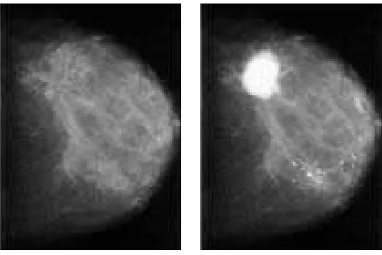
mam-(a) Normal breast (b) Cancerous breast

Figure 1.1: Typical mammogram

mography and clinical breast exam. However, ultrasound is not used alone for breast cancer screening. It does not produce an accurate image of the entire breast. MRI uses nuclear resonance to examine the breast, and there is promising evidence that it could eventually become a good tool for breast cancer screening [40]. Positron emission tomography detects how much sugar is being consumed by cells. Cancer cells tend to consume more sugar than normal tissue, which can help in identifying tumors. PET cannot provide a detailed enough image to find breast cancers in very early stages of development [13]. Therefore, it is currently not a promising option for breast cancer screening.

Computer Aided Detection (CAD) in mammography is a relatively new technology. The Food and Drug Administration (FDA) approved the first CAD device for film mammography in 1998 and expanded its approval to include the use of CAD for digital mammography detection in 2001.The technology is designed to provide an increased level of assistance to a radiologist when a mammography film is viewed. The computer software is designed to indicate areas in the mammogram that may be cancerous. However, the use of CAD as a second opinion, serves only to complement the interpreting radiologist, who must screen out the false indications of malignancies while accepting true lesions that might have been overlooked without CAD [20].

1.1

What are micro-calcifications

(a) Benign macrocalcifications are larger and randomly spread throughout the breast. No follow-up care is usually needed.

(b) Microcalcifications are small, ap-pear clustered and have irregular shapes. These may be a sign of

can-cer. Follow-up with more

mammo-grams and perhaps a biopsy are needed.

Figure 1.2: Calcifications in the breast

creeping out into the normal tissue will create either a fuzzy or spiky appearance along the outer edge (called "spiculated").

Another potential sign of cancer are small, bright white spots that are tiny calcium deposits which form in the breast as a woman ages. They are common and can result from a number of different things such as trauma to the breast and inflammation. There is no known relationship between the amount of calcium in a womans diet and breast calcifications. Calcifications are too small to be felt however a mammographic image is characterized by a high spatial resolution which is adequate to detect these subtle fine-scale signs. Most calcifications are benign and are actually quite common, with about half of all mammograms showing some. However, certain patterns of calcifications are suspicious so they must be looked at carefully as can be seen in Figure 1.2 . Tight clusters or lines of tiny calcifications (micro-calcifications) can be indications of cancer or precursors to cancer [52]. Individual MCs are sometimes difficult to detect because of the surrounding breast tissue, their variation in shape, orientation, brightness and size (typically, 0.05-1mm). This makes detecting MCs a complex and cumbersome task which requires highly specialized radiologists.

1.1.1

Types of calcifications

• Macro-calcifications are almost always benign (not cancer). They appear large and round on the

• Micro-calcifications are smaller and more numerous than the larger macro-calcifications. They are usu-ally benign, but can sometimes be a sign of cancer. The radiologist will look at the size, shape and distribution of the micro-calcifications to see if they are suspicious. More mammograms, an ultrasound study and a biopsy may be necessary. Suspicious micro-calcifications turn out to be cancer about 20 to 25 percent of the time.

• Sometimes it is hard to tell if micro-calcifications are cancer or not. These micro-calcifications are called

indeterminate.When this happens the radiologist may take more X-rays to help decide if the micro-calcifications are benign, probably benign, suspicious, or malignant. If they are probably benign, then there is a 98 percent chance that they are not cancer. However, if they are suspicious, more follow-up is needed.

1.2

Selection of algorithms for comparison

In the literature there are many methods that have explored the challenge of detection of micro-calcifications(MCs) in mammograms and here we seek to evaluate three of the best state of the art algorithms. In our study we will concentrate only on the problem of the detection of individual MCs rather than clusters. We shall also not investigate the problem of classifying them as benign/malignant.

Lee et al. [30] have described a prototype of a CAD system for detection of cancerous calcifications in mammograms. It employs fractal dimension to determine the roughness of an area which is different for calci-fication and normal background. To calculate the fractal dimension they used the Blanket Method developed by Mandelbrot and extended by Peleg for estimating the fractal dimension of a surface area. Bagci et al. [2] have employed the wavelet transform and adaptive filtering to get the error in predicting high pass components. MCs are then obtained by thresholding the wavelet coefficients based on their HOS( Higher Order Statistics) values . HOS test is a robust indicator of the Gaussianity of an area [19]. It is based on sample estimates of the first four moments of the prediction errors and the observation that wavelet transform has a Gaussian distribution of values except around the MCs. Wan Mimi et al. [54] have compared these two methods [19, 30] and reported the percentage of clusters detected to be 92% for [30] and 99% for [2] . Hence we chose Bagci’s approach [2] as the first method to be investigated.

all the other methods as shown in the FROC curves in [16]. Hence we chose this as the second method for our comparison.

Entropy thresholding forms another class of algorithms widely used in thresholding. It has also been used in detection of MCs in mammograms. Moti Melloul and Melloul et al. [38] have for the first time used a three dimensional co-occurrence matrix for threshold calculation. They obtained mean detection rates of 93.75% of true positives, 6.25% of false positives, and 2.0% of false negatives. It was reported to be better than three other state of the art algorithms that they used for comparison. Hence we chose this as the third algorithm for our investigation. Melloul et al. [38] have tested on the MIAS database (8 bit images of size 1024x1024), however we have tested it on the DSDM database (12 bit images). We have also compared its performance with three other entropy thresholding methods.

1.3

Synthesis of calcifications on mammograms

classi-1 2 1

2 4 2

1 2 1

Figure 1.3: Low pass filter used in synthesis of microcalcifications

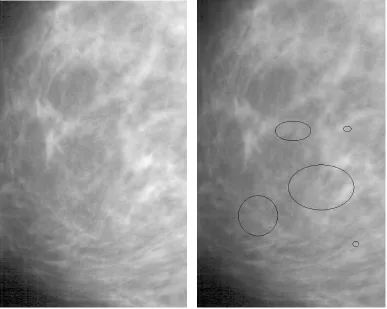
fied as uncertain. Further review of literature on simulated of microcalcifications can be found in [29]. Some authors have also tried to artificially construct the whole mammogram. These can be found in [48, 44, 46, 45]. Our effort is similar to that mentioned in [29] where we have a bank of real microcalcifications as marked by an experienced radiologist. Microcalcifications randomly chosen from the bank are placed at random locations over a normal mammogram. Low pass filtering around the border of the microcalcification blends it with the background. Figure 1.3 shows the filter used during this process. However this method is not fool proof since even normal mammograms can have microcalcifications. We have not attempted to simulate microcalcification clusters since we only deal with the problem of detection of individual microcalcifications rather than clusters. In Figure 1.4 and Figure 1.5 we can see the result of this procedure on two mammogram regions.

1.3.1

Organization of the thesis

Chapter 1 gives an introduction to CAD in breast cancer detection. It also gives a brief literature review and shows how were the three algorithms selected for comparison. It also describes a method for the synthesis of microcalcifications on normal mammograms.

Chapter 2 describes the wavelet filtering based algorithm mentioned in [2] and a brief literature review related to use of wavelets in detection of MCs. In [2] authors rank the locations by its HOS value but do not provide any statistics such as false positive or true positive detection rate. We have extended their approach by selection of threshold using minimum cross entropy thresholding as explained in the section 3.1.1.

Chapter 3 describes entropy thresholding based methods to detect microcalcifications. We compare the three dimensional co-occurrence matrix based algorithm mentioned in [38] with three other entropy threshold-ing algorithms and select the best performthreshold-ing algorithm. The selected algorithm is then used for the detection of microcalcifications. It also gives a brief literature review about the application of similar information theoretic measures in thresholding.

(a) Normal mammogram without any microcalcifica-tion

(b) After addition of microcalfications

(a) Normal mammogram without any microcalcification (b) After addition of microcalfications

Chapter 2

Adaptive Wavelet Filtering

The theory of wavelets provides a common framework for numerous techniques developed independently for various signal and image processing applications. For example, multiresolution image processing, used in computer vision, subband coding, developed for speech and image compression, and wavelet series expansions, developed in applied mathematics, have been recently recognized as different views of a single theory. The classical approach for the analysis of non-stationary signals is the short-time Fourier transform (STFT) or Gabor transform. With the advent of wavelet transform (WT), short windows at high frequencies and long windows at low frequencies can be used to provide better signal resolution than the STFT. The Wavelet transform can also be seen from a signal decomposition view point. In this case, a signal is decomposed onto a set of basis functions which are called wavelets and are the core of wavelet analysis. These basis functions are obtained from a single mother wavelet by dilations and contractions (scalings), as well as translations or shifts. An excellent review of these techniques and concepts can be found in [55] where it is also shown that wavelet decomposition is closely related to multirate signal processing techniques. A particular wavelet decomposition relates to filter banks and can be the basis for subband coding schemes used in speech and image compression.

micro-calcifications tend to appear. Clusters of MCs are then detected by performing a third order HOS Gaussianity test [23]. Wang and Karayiannis [55] have given an excellent review of wavelet theory and its application to images. According to their approach MCs are extracted from mammograms by suppressing the subband of the wavelet-decomposed image that carries the lowest frequencies and contains smooth (background) information. Only the high frequency components are used to reconstruct the image. The visibility of MCs is improved by using a nonlinear thresholding method to enhance the histogram of the resulting mammograms. Wan Mimi Diyana et al. have mentioned in [15] a wavelet based approach which used Higher Order Statistics(HOS). HOS test has been first mentioned in the literature in [53] and has been beautifully described in [34]. Below we outline normal subband decomposition and adaptive subband decomposition which has been explored in this work.

2.1

Wavelet based representation of images

2.1.1

Normal subband decomposition

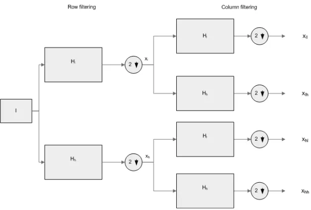
Wavelet-based image decomposition can be interpreted as an image filtering process. Normal wavelet sub-band decomposition has been illustrated in Figure 2.1. For a given image I of size 2nx 2n wavelet-based subband decomposition can be performed as follows: the wavelet filters hl(n)and hh(n)are applied to the rows

of the image I. The filter hl(n)is a low-pass filter with frequency response Hl(ω)and hh(n)is a high-pass

filter with frequency response Hh(ω). By filtering the image I with Hl(ω), we obtain low-frequency

informa-tion(background). By filtering the image with Hh(ω), we obtain the high-frequency information(edges). After

downsampling by a factor of two, we obtain two subbands: xl and xh. Since we downsample by a factor of

two in the horizontal direction of each subband, the size of these two downsampled subbands is 2nx 2n−1(see Figure2.1). The filters are then applied to the columns of the subbands xland xh, and the following four

sub-bands are obtained , xll, xlh, xhland xhh. Since we now downsample by a factor of two in the vertical direction

of each subband, the four subbands have gone through downsampling by a factor of two in both directions and the final size of each subband is 2n−1x 2n−1(see Figure 2.1).

The subband xll contains the smooth information and the background intensity of the image and the

sub-bands xll, xlhand xhlcontain the detail information of the image. The subband xll corresponds to the lowest

frequencies, xlhgives the horizontal high frequencies (vertical edges), xhlgives the vertical high frequencies

Figure 2.1: Two dimensional subband decomposition using wavelet filters

2.1.2

Adaptive subband decomposition

Bagci et al. [2] have used the adaptive wavelet structure proposed by Ömer Nezih Gerek et al. in [18] for image compression. They have shown that it works better than normal subband decomposition especially at the regions that are not as bright or significant as others. In this structure (Figure 2.2) the low band signal xlis

obtained by down-sampling the original signal, x and consists of only even samples. The high pass component xhis obtained through an adaptive filter structure. The sequence x2is a shifted and downsampled version of the original signal x and consists of only odd samples. Next ˆx2the estimate of x2is obtained using xland filter0w0

as shown in equation 2.1. The adaptive FIR estimator used is obtained by predicting the odd samples x2from the even samples xlas follows:

ˆ x2=

k=N

∑

k=−N

wn,kxl(n−k) = k=N

∑

k=−N

wn,kx(2n−2k) (2.1)

The filter coefficients w0_n,ks are updated using an LMS type algorithm as follows:

ˆ

w(n+1) =wˆ(n) +µν˜ne(n) kν˜nk2

(2.2)

where ˆw(n) = [wn,−N, . . . ,wn, . . . ,wn,N]is the weight vector and ˜νn= [xl(n−N),xl(n−N+1), . . . ,xl(n+N−

Figure 2.2: Adaptive subband decomposition structure

uni-dimensional signal. The extension of this adaptive filter bank structure to two dimensions is done in the same way as normal subband decomposition in section 2.1.1. Initially rows are filtered and the obtained images are column filtered thus again giving four subimages xll, xlh,xhland xhl. Low-low image xllcan be ignored in

analysis as it gives background information and during the experiments it was observed that xhhdid not contain

any information relevant to the current problem of detection of microcalcifications. Hence xlh and xhlhave

been used as in [2].

2.1.3

HOS test

Bagci et al. [2] have mentioned that MCs occur as isolated bright spots on the mammogram hence they correspond to local maxima on the image. Fourth order statistics or Kurtosis which we shall use in identification of MCs can be represented by

H=γ4=

E{[x−E(x)]4_}

(E{[x−E(x)]4_})2−3 (2.3)

Figure 2.3: 8 search directions around the center pixel

calculating the HOS values on the actual image as mentioned in [2]. However average maximum for positive positions i.e. microcalcifications was greater for wavelet image, hence it was decided to work with the wavelet image. Some of the true MCs had HOS values less than non-MC which makes it difficult to decide upon a threshold.

2.1.4

Algorithm

Below we outline the steps in this algorithm:

• Bagci et al. [2] have outlined a pre-processing scheme to determine the location of maxima. These

constitute a subset which dictates the positions where fourth order HOS test is carried out. For this purpose we extract a 5x5 window around each pixel and if the maximum is 1.1 times the minimum value in the window then that pixel is recorded as a maxima. If it does not satisfy this criteria but pixel value is 10% greater than the minimum value and greater than or equal to the maximum value of the neighbouring pixels then we check the following condition: check the two pixels in each 8 directions around the pixel as shown in the Figure 2.3. If the value of the center pixel is 1.05 times greater than at least one of the two pixels in each direction then the point is marked as possible microcalcification region.

• Obtain the wavelet transform of the input image using the adaptive subband structure explained in section

2.1.2. Thus we get the quarter sized wavelet image e[m,n] = (|xlh|+|xhl |)[m,n]. It is also

pre-thresholded with a small threshold0t0, which avoids peaks due to the background which can affect the entropy thresholding process.

• Estimate the fourth order statistic, H, in a MxM window around each maximum location in the image at

image then we search at the location m = round(i/2), n = round(j/2) in the image e[m,n]. H is estimated as shown below

H(I1,I2,I4) =I4+2I14−3I22 (2.4)

Ik=

1 M+N

M

∑

m=1

N

∑

n=1

ek[m,n],k=1,2,3,4 (2.5)

• In the method mentioned in [2] first the local maximas of the image are detected as above and ranked

according to a high order statistical (HOS) test performed over the subbands obtained by the adaptive wavelet transform. No statistical results have been provided in [2] terms of false positives or ROC curve against which one can evaluate the efficacy of their algorithm. However we differ from their method as we calculate a threshold T, using the entropy thresholding method mentioned in [33]. Presence of a microcalcification is determined if H is greater than or equal to this threshold. Thus the output of our procedure shows locations of MCs which is then compared with the truth. This enables us to obtain a ROC curve and compare it with other algorithms mentioned in this work.

2.1.5

Experimental results

Parameters Fraction of true positives detected False positives per image

µ=2, t=2 0.19 147.91

µ=1, t=2 0.31 49.41

µ=0.1, t=2 0.32 36.77

µ=0.2, t=−20 0.33 35.18

µ=0.2, t=0 0.33 35.18

µ=0.2, t=0.5 0.33 35.18

µ=0.2, t=2 0.33 35.18

µ=0.2, t=10 0.33 35.18

µ=0.2, t=20 0.33 35.18

µ=0.5, t=2 0.32 33.86

Table 2.1: Results with Wavelet based approach for varying µ and pre-threshold0t0

Parameters Fraction of true positives detected False positives per image

µ=2, t=2 0.29 86.4

µ=1, t=2 0.82 25.7

µ=0.1, t=2 0.82 34.7

µ=0.2, t=−20 0.84 32.1

µ=0.2, t=0 0.84 32.1

µ=0.2, t=0.5 0.84 32.1

µ=0.2, t=2 0.84 32.1

µ=0.2, t=10 0.84 32.1

µ=0.2, t=20 0.84 32.1

µ=0.5, t=2 0.76 26.3

Chapter 3

Entropy thresholding

Shannon [49] defined the entropy of a system as a function of the probability of occurrence of different states of the system. If a system has n different states with probability of occurrence pi,i=1,2, . . . ,n,∑ni=1pi=1,

then the gain in information from the occurrence of the event i is defined as4I=−log₂pi.The expected value

of such a gain in information is defined as the entropy of the system. Thus the entropy H of the system is: H=−∑n

i=1pi. Let F= [f(x,y)]PxQwhere f(x,y)is the gray value at (x,y); f(x,y) =∈GL={0,1, . . .,L−1},

the set of gray levels. Let Ni be the frequency of the gray level i. Then∑Li=−11Ni=PxQ=N. Following

Shannon’s definition of entropy, entropy of the image histogram can be defined as

H=−

L−1

∑

i=0

pilog2pi; pi=Ni/N (3.1)

for the image segmentation problem. Thus different images with identical histograms will result in same entropic value in spite of their different spatial distributions of gray levels. N.R. Pal et al. [41] have given a different formulation of entropy for images. We know that in an image pixel intensities are not independent of each other. This dependency of pixel intensities can be incorporated by considering sequences of pixels to estimate the entropy. In order to arrive at the expression of entropy of an image the following theorem due to Shannon can be stated:

Theorem: Let p(si)be the probability of a sequence si of gray levels of length q, where a sequence siof

length q is defined as a permutation of q gray levels. Let us define

H(q)=−1

where the summation is taken over all gray level sequences of length q. Then H(q)is a monotonic decreasing function of (q) and limq→∞H(q)_{=H,the entropy of the image.}

For different values of q we get different orders of entropy.

Case 1: q = 1 , i.e. sequence of length one. If q = 1 we get H(1)=−∑L−1

i=0 pilog2pi, where pi is the

probability of occurrence of the gray level i. Such an entropy is a function of the histogram only and it may be called the “global entropy” of the image. Therefore different images with identical histograms would have same H(1)value irrespective of their contents.

Case2: q = 2, i.e. sequences of length two. Hence, H(2)=−∑_iL₌−₀1pilog2pi, where si is a sequence of

gray level of length two,=∑i∑jpi jlog2pi j, where pi jis the probability of co-occurrence of the gray levels i

and j. Therefore H(2)can be obtained from the co-occurrence matrix, defined in section 3.1.2. H(2)takes into account the spatial distribution of gray levels. Therefore, two images with identical histograms but different spatial distributions will result in different entropy, H(2)_{values. Expressions for higher order entropies( q >}

2) can also be deduced in a similar manner. H(i)_{, i≥2, may be called the “local entropy of the image”. The}

power of the gray level co-occurence approach is that it characterizes the spatial interrelationships of the gray levels in a textural pattern and can do so in a way that is invariant under monotonic gray level transformations. Its weakness is that it does not capture the shape aspects of the gray level primitives. Hence it is not supposed to work well for textures composed of large area primitives. Also it cannot capture the spatial relationships between primitives that are regions larger than a pixel. In section 3.1.2 more details about the approach followed by Pal et al. [41] have been given.

by experiment that visual inspection was consistent with uniformity and shape measures. Brink & Pendock [6] use cross-entropy to determine the appropriate threshold. They also compare it with metric measures such as cross correlation,χ2_{measure of discrepancy and show that use of a correlation measure for thresholding} is valid (in terms of maximum entropy theory) only if the distributions are normal and the first moment is preserved. [12, 25, 54] use two dimensional co-occurrence matrix for entropy thresholding. [58] have reported the superiority of two dimensional histogram instead of co-occurrence for entropy thresholding. Kurani et al. [28] investigate a new approach to the co-occurrence matrix currently used to extract textural features: co-occurrence matrices for volumetric data. It is used to calculate volumetric texture descriptors that can be used for segmentation and classification of soft tissues in CT studies. C.H. Li & P.K.S. Tam [33] derive a fast iterative method for minimum cross entropy thresholding which accurately locates the threshold while significantly reducing the computational cost.

3.1

Algorithms

We have compared four entropy thresholding techniques and applied the best one for the detection of micro-calcifications on mammograms. Below we describe each of the four techniques.

3.1.1

Minimum cross entropy thresholding

This algorithm has been described by Li et al. in [33]. For a histogram h defined on the gray level range [0,L-1] , the zeroth and the first moments of the foreground and background portions of the thresholded histogram are respectively,

m0a(t) =

t−1

∑

i=0

h(i) mob= L−1

∑

i=t

h(i) (3.3)

m1a(t) =

t−1

∑

i=0

ih(i) mob= L−1

∑

i=t

ih(i) (3.4)

The portions’ means are defined as

µa(t) =

m1a(t) m0a(t)

µb(t) =

m1b(t) m0(t)

(3.5)

η(t) =−m1a(t)log(µa(t))−m1b(t)log(µb(t)) (3.6)

Thus the optimal threshold is given by the minimizer of equation 3.6, top=arg mintη(t).

3.1.2

Two dimensional co-occurrence matrix based

N.R. Pal, S.K. Pal [41] is one of the earliest works in entropy thresholding. It is based on maximizing the conditional entropy of object and background. Suppose an image has two distinct portions, the object X and the background Y. Suppose the object consists of the gray levels {xi} and the background contains the gray

levels {yi}. The conditional entropy of the object X given the background Y, i.e. the average amount of

information that may be obtained from X given that one has viewed the background Y, can be defined as

H(X/Y) =−

∑

xi∈X

∑

yj∈Y

p(xi/yj)log2p(xi/yj) (3.7)

Similarly the conditional entropy of the background Y given the object X is defined as

H(X/Y) =−

∑

xi∈X

∑

yj∈Y

p(yj/xi)log2p(yj/xi) (3.8)

An additional constraint is imposed that yjand xihave to be adjacent.

Algorithm 1

Based upon the above formulation the co-occurrence matrix of an image I of size PxQ and L gray levels is an LxL dimensional matrix T= [ti j]LxLthat gives an idea about the transition between adjacent pixels. Each entry

in the matrix ti jgives the number of times the gray level j follows the gray level i in some pattern. Depending

upon different patterns different definitions of co-occurrence matrix are possible. It has been reported in [41] that consideration of both horizontal and vertical transitions allows all the edges to participate in the threshold selection. Thus ti jis defined as follows:

ti j= P

∑

l=1

Q

∑

k=1

δ (3.9)

where

δ=1,if

          

f(l,k) =i and f(l,k+1) =j or

f(l,k) =i and f(l+1,k) =j;

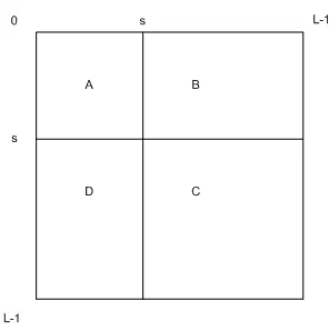
Figure 3.1: Quadrants of co-occurrence matrix

The probability of co-occurrence pi jof gray levels i and j therefore can be written as

pi j=ti j

,

∑

i

∑

ti j (3.11)

If s, 0≤s≤L-1 is a threshold, then ’s’ partitions the co-occurrence matrix into four quadrants, namely A,B,C

and D as seen in Figure 3.1. Let us define the following quantities

PA=

s

∑

i=0

s

∑

j=0

pi j, PB=

s

∑

i=0

L−1

∑

j=s+1 pi j

PC=

L−1

∑

i=s+1

L−1

∑

j=s+1

pi j, PD=

L−1

∑

i=s+1

s

∑

j=0 pi j

(3.12)

Normalizing the probabilities within each individual quadrant, such that the sum of the probabilities of each quadrant equals one, we get the cell probabilities for different quadrants:

pA_{i j} = pi j PA

= ti j

, _L−1

∑

i=0

L−1

∑

j=0 ti j

!

s

∑

i=0

s

∑

j=0

(

ti j

,

L−1

∑

i=0

L−1

∑

j=0 ti j

) (3.13)

= _s ti j

∑

i=0

s

∑

j=0 ti j

for 0≤i≤s, 0≤j≤s

pB_{i j} = pi j PB

= ti j

s

∑

i=0

L−1

∑

j=s+1 ti j

(3.14)

for s+1≤i≤L-1, s+1≤j≤L-1

and

pC_{i j} = pi j PC

= ti j

L−1

∑

i=s+1

L−1

∑

j=s+1 ti j

(3.15)

for s+1≤i≤L-1, s+1≤j≤L-1

pD_{i j} = pi j PD

= _L−1ti j

∑

i=s+1

s

∑

j=0 ti j

(3.16)

for s+1≤i≤L-1, s+1≤j≤L-1

Now the second order local entropy of the background can be defined as

HA(s) =−

1 2

s

∑

i=0

s

∑

j=0

pA_{i j}log₂pA_{i j}. (3.17)

Similarly the second order entropy of the object can be written as

HC(s) =−

1 2

L−1

∑

i=s+1

L−1

∑

j=s+1

pC_{i j}log₂pC_{i j}. (3.18)

Hence the total second order local entropy of the object and the background can be written as

HT(s) =HA(s) +HC(s). (3.19)

Algorithm 2

This algorithm is based on the concept of conditional entropy. Suppose ’s’ is an assumed threshold then pixels with gray level values ranging from 0 to s correspond to the background while the remaining pixels with gray levels between s+1 to L-1 constitute the object. Let ti jbe an entry of the quadrant B then ti jgives the number of

transitions such that i belongs to the background and j belongs to the object, and i and j are adjacent. Therefore,

H(object/background)=H(O/B) =−

L−1

∑

i=s+1

s

∑

j=0

pD_{i j}log₂pD_{i j} (3.20)

and

H(background/object)=H(B/O) =−

s

∑

i=0

L−1

∑

j=s+1

pB_{i j}log₂pB_{i j} (3.21) Now the conditional entropy of the image is

HT(s) = (H(O/B) +H(B/O))/2. (3.22)

In order to get the threshold for object-background classification HT is maximized with respect to ’s’ and that

maximum value of ’s’ is the selected threshold.

3.1.3

Three dimensional co-occurrence matrix based

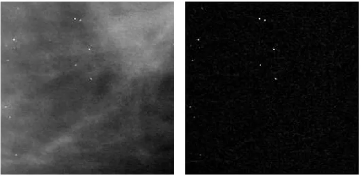
Melloul et al. [38] have described an algorithm similar to that in [41] with the difference based in the use of three dimensional co-occurrence matrix for thresholding and tophat morphological filter as a pre-processor. Tophat filtering removes objects which are larger than the kernel which in this case is of size 5x5. It involves morphological gray scale opening of the input image. The opened image is then subtracted from the input image. The effect of this pre-processing can be seen in the Figure 3.2. A three dimensional co-occurrence matrix of an image is an LxLxL dimensional matrix, T = [ti jk]LxLxLwhich contains information regarding

separating background and microcalcifications is the one which gives maximum sum of the entropies. An entry ti jkof the 3D co-occurrence matrix is defined by

ti jk= M

∑

m=1

N

∑

n=1

δ(m,n) (3.23)

where

δ(m,n) =

      

1 if f(m,n)=i and f(m,n+1)=j and f(m+1,n)=k

0 otherwise

(3.24)

The two volume objects (O) and background (B) can be separated in the 3D co-occurrence matrix defined by the equation 3.23. Let t∈G be the threshold of the two groups the foreground and background in the image

B={(i,j,k)|0<i<t,0<j<t,0<k<t}

O={(i,j,k)|t+1<i<L−1,t+1<j<L−1,t+1<k<L−1}

Microcalcifications are associated with the foreground and are pixels with gray levels greater than or equal to the threshold. Background is associated with the pixels which are below the threshold. The probabilities associated with each volume are defined by

PB(t) = t

∑

i=0

t

∑

j=0

t

∑

k=0

pi jk (3.25)

PO(t) = L−1

∑

i=t+1

L−1

∑

j=t+1

L−1

∑

k=t+1

pi jk (3.26)

The probabilities in each volume are defined by normalization

pB_{i jk}= pi jk PB

= _t ti jk

∑

i=0

t

∑

j=0

t

∑

k=0 ti jk

(3.27)

pO_{i jk}= pi jk PO

= ti jk

L−1

∑

i=t+1

L−1

∑

j=t+1

L−1

∑

k=t+1 ti jk

The background entropy HB(t)and the object entropy HO(t)are computed on the volumes B and O which

each are defined by

HB(t) =−

1 2_(i,

∑

B

i jlog2pBi j (3.28)

HO(t) =−

1 2₍

∑

i,j)∈O

pO_{i j}log₂pO_{i j} (3.29)

Note that HBand HOare determined by the threshold, thus they are a function of t. By summing up the entropies

of the object and the background, the image entropy can be obtained by

H(t) =HB(t) +HO(t). (3.30)

This algorithm selects a threshold which maximizes H over t. The optimal threshold is value of t which maximizes the image entropy.

3.1.4

Experiments

Experimental comparison of entropy thresholding algorithms

Here we have compared three-dimensional entropy thresholding in [38], two dimensional algorithms in [41] and minimum cross entropy based thresholding in [33]. Figure 3.2 shows the 12-bit test input image before and after filtering with the morphological tophat filter mentioned in [38]. Both images are gray scale and microcalcifications are easily visible in the tophat filtered image, thus it appears to be an easy job to segment microcalcifications from the background. For all the algorithms the tophat filtered image is pre-thresholded with the same threshold (= 75) and first few values in the histogram/co-occurrence matrix are ignored. This is because background occupies a major portion of the mammogram and it gives rise to peaks in the early part of the histogram which clouds peaks due to breast anatomy.

Figure 3.3 shows output with two algorithms from [41] when the input image is scaled to 8-bit. As already mentioned in their paper algorithm-2 (section 3.1.2) outperforms algorithm-1 (section 3.1.2). For comparison Figure 3.4 shows the output for both algorithm-1 and algorithm-2 when images are not scaled. This goes to show that both the algorithms are highly sensitive to scaling. This could be because the co-occurrence matrix is highly sparse in the unscaled case.

(a) Input image for comparison (b) Input image after tophat filtering

Figure 3.2: Input image for comparison of thresholding algorithms

Parameters Fraction of true positives detected False positives per image

t=25 1 13120.5

t=50 0.98 8180.32

t=75 0.87 2742

t=100 0.73 373

t=125 0.48 11.73

t=150 0.4 5.91

t=175 0.37 3.45

t=200 0.35 2.45

Table 3.1: Results with cross entropy based approach with variation of pre-threshold0t0

based methods which fail in case of images with greater brightness resolution. This can probably be attributed to the sparsity of the co-occurrence matrix with increasing grayscale resolution. Increased resolution will also result in an almost flat histogram.

Experiments with the cross entropy based thresholding algorithm

We chose the cross entropy based thresholding algorithm to be compared with other approaches mentioned

in this work since it worked best as shown in section 3.1.4. Here too we threshold the image after pre-processing (in this case a tophat morphological filter) with a pre-threshold0t0. In section 2.1.5 also we threshold the image after filtering with the adaptive wavelet filter. This threshold is varied to obtain various performance points. Table 3.1 shows its performance as we vary the pre-threshold0t0. This is again done to avoid peaks due to the background which could be peaks due to the breast anatomy.

(a) Output with two dimensional co-occurrence matrix based thresholding for algorithm 1

(b) Output with two dimensional co-occurrence matrix based thresholding for algorithm 2

Figure 3.3: Thresholding the image in Figure 3.2 using algorithms in [41]

(a) Output with two dimensional co-occurrence matrix based thresholding for algorithm 1 without scaling

(b) Output with two dimensional co-occurrence matrix based thresholding for algorithm 2 without scaling

(a) Output with cross entropy based thresholding (b) Output with three dimensional co-occurrence ma-trix based thresholding

Figure 3.5: Thresholding the image in Figure 3.2 with scaling between 0-255

(a) Output with cross entropy based thresholding with-out scaling

(b) Output with three dimensional co-occurrence ma-trix based thresholding without scaling

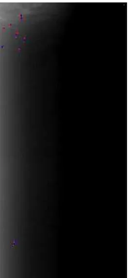
Figure 3.7: Output with cross entropy based approach for image which gave worst performance with the wavelet approach. False positives = 3, False negatives = 4 (blue - true MC, red - detected MC)

that whereas wavelet filtering achieves a maximum detection percentage of 33% with 35.18 false positives per image, cross entropy based algorithm detects 48% of MCs with only 11.73 false positives per image. Also in Figure 3.7 we can see its output for the same image which gave worst performance for the wavelet based approach (Figure 2.5). It is apparent that it outperforms the wavelet approach since it has only 3 false positives and 4 false negatives as against 285 false positives and 6 false negatives with the wavelet approach. In Figure 3.8 we can see an instance when it does not work well.

This algorithm also offers the advantage of a handle in terms of pre-threshold0t0 which can be tuned to achieve higher detection rates, though at the cost of more false positives per image. In Figure 3.9 we can see the ROC curve for wavelet and cross entropy based methods on absolute as well as logarithmic scale for real images. ROC curve is a plot of percentage/fraction of true positives detected versus false positives per image.

0 5000 10000 15000 0.1

0.2 0.3 0.4 0.5 0.6 0.7 0.8 0.9 1

False positives per image

Fraction of true MCs detected

Absolute scale

Cross entropy Wavelet

100 105

0.1 0.2 0.3 0.4 0.5 0.6 0.7 0.8 0.9 1

False positives per image

Fraction of true MCs detected

Log scale on X axis

Cross entropy Wavelet

Parameters Fraction of true positives detected False positives per image

t=25 0.98 7800.5

t=50 0.88 1628.4

t=75 0.77 12.6

t=100 0.68 6.1

t=125 0.66 4.7

t=150 0.62 3.7

t=175 0.56 3

t=200 0.5 2.7

Table 3.2: Results obtained for cross entropy based algorithm with simulated microcalcifications

Chapter 4

Support Vector Machines

Burges [7] has provided an excellent tutorial for Support Vector Machines and explains the key concepts in a very lucid language. The description that follows has been taken from the same. SVM’s have provided a new approach to the problem of pattern recognition with clear connections to the underlying statistical learning theory. They differ radically from comparable approaches such as neural networks: SVM training always finds a global minimum and has simple geometric interpretation. The problem which drove the initial development of SVMs occurs in several guises- the bias variance trade-off, capacity control, overfitting - but the basic idea is the same. For a given learning task with a given amount of training data, the best generalization performance will be achieved if the right balance is struck between the accuracy attained on that particular training set and the “capacity” of the machine. A machine with too much capacity is like a botanist with a photographic memory who when presented with a new tree concludes that it is not a tree because it has a different number of leaves from anything he has seen before; a machine with too little capacity is like his lazy friend who says that if it is green then it must be a tree. Neither can generalize well. The formulation and exploration of these concepts led to a path breaking development in the theory of statistical learning theory. This theory is the principle of

structural risk minimization (SRM) (Vapnik, 1979). It grew out of considerations of under what circumstances, and how quickly the mean of some empirical quantity converges uniformly to the true mean (that which would be calculated from an infinite amount of data), as the number of data points increases. We will briefly try to cover this principle since this forms the backbone of SVMs.

Suppose we have a machine whose task is to learn the mapping xi7→yi. The machine is actually defined by

parameterα. The expectation of the test error for a trained machine is therefore:

R(α) =

Z

1

2 |y−f(x,α)|dP(x,y) (4.1)

The quantity R(α)is called the expected risk or just the risk and this is the quantity that we are ultimately interested in. The “empirical risk” Remp(α)is defined to be just the measured error rate on the training set (for

a fixed, finite number of observations):

Remp(α) =

1 2l

l

∑

i=1

|yi−f(xi,α)| (4.2)

where l is the number of observations. The quantity 1₂|yi−f(xi,α)|is called the loss. Suppose we define our

problem such that the loss can only be either 0 or 1. Now choose someηsuch that 0≤η≤1.Then for losses taking these values with probability 1−η, the following bound holds (Vapnik, 1995):

R(α)≤Remp(α) +

s

_{h(log 2l/h) +1)−log(}η_/4)

l

(4.3)

where h is a non-negative integer called the Vapnik Chervonenkis (VC) dimension and is a measure of the notion of capacity above. The second term on the right in is called the “VC confidence”. It is a monotonically increasing function of h for any value of l.Given some selection of learning machines whose empirical risk is zero, one wants to choose that machine whose associated set of functions has minimal VC dimension.

We can now summarize the principle of SRM. The VC confidence term in equation (4.3) depends on the chosen class of functions whereas the empirical risk and actual risk depend on the one particular function chosen by the training procedure. We would like to find that subset of the chosen functions, such that the risk bound for that subset is minimized. One cannot arrange things so that the VC dimension varies smoothly, since it is an integer. Instead introduce a “structure” by dividing the entire class of functions into nested subsets. For each subset we must be able to compute h, or to get a bound on h itself. SRM then consists of finding that subset of functions which minimizes the bound on the actual risk. This can be done by simply training a series of machines one for each subset where for a given subset the goal of training is simply to minimize the empirical risk. One then takes that trained machine in the series whose sum of empirical risk and VC confidence is minimal.

Figure 4.1: Linear support vector classifier with separable data. Support vectors are circled. (From [7])

4.1

Review of support vector machine classifiers

4.1.1

Linear SVMs

SVMs are best understood in the linear case. We assume that the training data is linearly separable i.e. there exists a hyperplane of the form w•x+b=0,where w is normal to the hyperplane,|b|/kwkis the perpen-dicular distance from the hyperplane to the origin,kwkis the Euclidean norm of w and yi∈[+1,−1]is class

label or identifier. Since this hyperplane separates the data we can say:

w•xi+b≥1 for yi= +1 (4.4)

w•xi+b≥1 for yi=−1 (4.5)

These can be combined into one set of inequalities:

yi(w•xi) +b≥0 ∀i (4.6)

Now consider the points for which the equality in Eq. (4.4) holds. These points lie on the hyperplane H1: xi•w+b=1 with normal w and perpendicular distance from the origin|1−b|/kwk.Similarly, the

points for which the equality in Eq. (4.5) holds lie on the hyperplane H2: xi•w+b=−1 with again the normal

being w and perpendicular distance from the origin| −1−b|/kwk.Hence the margin, distance between the positive and negative hyperplanes is 2/kwk.Note that H1and H2are parallel (they have the same normal) and that no training points fall between them. Thus one can find the pair of hyperplanes which gives the maximum margin by minimizingkwk2_{, subject to constraints (Eq. 4.6). For a given training set, while there may exist} many hyperplanes that separate the two classes, the SVM classifier is based on the hyperplane that maximizes the separating margin between the two classes (Figure 4.1) . This hyperplane can be found by minimizing the margin given by

J(w) =1 2w

T_w=kwk2 _(4.7)

Figure 4.2: Linear support vector classifier with non-separable data. Support vectors are circled. (From [7])

variablesξi,i=1, . . . ,l in the constraints. Now the equations (4.5) and (4.4) look like:

xi•w+b≥+1−ξi for yi= +1

xi•w+b≥ −1−ξi for yi=−1

ξi≥0∀i

(4.8)

Thus for an error to occur the correspondingξimust exceed unity, so∑iξiis an upper bound on the number

of training errors. Hence the objective function is modified tokwk2_/2+C(∑

iξi)kwhere C is a parameter to

be chosen by the user, a larger C corresponding to assigning a higher penalty to errors. This situation can be visualized in Figure 4.2.

4.1.2

Nonlinear support vector machines

In section 4.1.1 we assume that the decision function is a linear function of the data. So how do we deal with the case when it is not so obvious (Figure 4.2)? This is accomplished by mapping the data to some other (possibly infinite dimensional) Euclidean space using a mapping

Φ: Rd7→

H

In the solution of Eq. (4.7) (refer [7] for details) with constraints (4.4) & (4.5); the data xionly appears in the

kernel function K such that K(xi,xj) =Φ(xi)•Φ(xj),we will only need to use K in the training algorithm and

would never need to explicitly even know whatΦis. For example the radial basis kernel:

K(xi,xj) =e−kxi−xjk

2_/2σ2

.

can be shown to satisfy the required properties for such a kernel. In this particular example

H

everywhere in the training algorithm, it will easily produce a support vector machine which lives in an infinite dimensional space. For example for kernels of the form K = (xi•xj)p, a dot product in

H

computations of order( dL+p−1 p

)operations, whereas the computation of K= (xi•xj)requires only O(dL)

operations (dL being the dimension of the data). It is this fact that allows us to construct hyperplanes in

these very high dimensional spaces and yet be left with a tractable computation. Thus SVMs circumvent both forms of the “curse of dimensionality”: the proliferation of parameters causing intractable complexity, and the proliferation of parameters causing overfitting.

Some kernels used in Nonlinear SVMs

An SVM is largely characterized by the choice of its kernel, thus SVM links the problems they are designed for with a large body of existing work on kernel methods. But perhaps this kernel is also its biggest limitation. Once the kernel is fixed, SVM classifiers have only one user-chosen parameter (the error penalty) but the best choice of kernel for a particular problem is still a research issue. A second limitation is speed and size, both in training and testing. Training for very large datasets (millions of support vectors) is an unsolved problem. Below are examples of kernels used for pattern recognition problems:

K(x,y) = (x•y+1)p _(4.9)

K(x,y) =e−kx−yk2/2σ2 (4.10)

K(x,y) =tanh(κx•y−δ) (4.11)

identical. The parameters such asσare determined during the training phase.

Now the question arises that how does one say if there exist a pair{

H

above and for which there does not? The answer is given by the Mercer’s condition: There exists a mappingΦ and an expansion

K(x,y) =

∑

i

Φ(x)iΦ(y)i (4.12)

if and only if, for any g(x)such that

R

g(x)2_{dx is finite then}

Z

K(x,y)g(x)g(y)dxdy≥0. (4.13)

A simple way to express the same condition is that any kernel which can be expressed as K(x,y) =∑∞p=0cp(x•

y)p_{, where c}

pare positive real coefficients and the series is uniformly convergent, satisfies Mercer’s condition.

4.2

Successive enhancement learning algorithm

Training a SVM classifier that operates on the whole mammogram is difficult due to the overwhelming number of negatives and very few positives (microcalcifications). El Naqa et al. [16] have described a SEL (Successive Enhancement Learning) algorithm to this purpose which selects only the most representative negative samples while keeping the training set within tolerable limits. It has been outlined below:

1. Extract an initial set of training examples from the available training images. Let Z={(x1,y1),(x2,y2), . . . ,(xl,yl)}

denote the resulting set of training samples.

2. Train a SVM classifier with Z.

3. Apply the resulting classifier to all the mammogram regions (except those in Z) in the available training images and record the “MC absent” locations that have been misclassified as “MC present”.

4. Gather N new input examples from the misclassified “MC absent” locations; update the set by replacing “MC absent” examples that have been classified correctly by the classifier with the newly collected “MC absent” examples.

5. Re-train the SVM classifier with the updated set Z.

6. Repeat steps 3-5 until convergence is achieved.

randomly from the set of misclassified “MC absent” locations. The convergence in step 6 was monitored by its error over another set of “MC absent” positions selected randomly from the training set such that they did not overlap with the existing “MC absent” samples.

4.3

Experiments

4.3.1

Training phase

(a) Input image before high pass filtering (b) Input image after high pass filtering

Figure 4.3: Effect of high pass filtering (length = 41, cut off frequency = 0.125) on mammogram

Figure 4.4: Selection of positive samples from the neighbourhood of a MC. Center pixel is shown black and extra positive locations selected are shown as gray

error we collect windows of size MxM (M = 9), centered on a 3x3 neighbourhood as shown in the Figure 4.4. Negative samples (pixels identified as MC absent, yi=−1) number twice that of positive samples and were

selected randomly such that they don’t overlap. So for a total of 677 positive samples we collect a total of 1354 negative samples. This constitutes the initial data set Z in step 1 in the SEL algorithm (section 4.2). A SVM classifier was trained on this data with radial basis function kernel using ’Spider’, a Matlab package provided by the Max Planck Institute of Biological Cybernetics, Tuebingen, Germany. Parameters obtained after training wereσ=1 and C=1000 (as in Eq. 4.10). This was followed by repeating steps 3-6 in the SEL algorithm till the generalization error (measured over an exclusive set of negative samples as explained in section 4.2) was sufficiently low. Figure 4.5 shows the variation of generalization error against number of iterations with negative sample size twice of that of the positive sample size. After nine iterations it achieves an error rate of 0.61% with 467 support vectors.

We also experimented with negative sample size being ten times the size of positive samples, however it gave no significant improvement in performance along with an increase in number of support vectors to 608. Hence we decided against taking this big a sample size since with an increase in number of support vectors the testing time also increased.

4.3.2

Testing phase

1 2 3 4 5 6 7 8 9 0.005

0.01 0.015 0.02 0.025 0.03

Iteration

Generalization error

Figure 4.5: Variation of error with the number of iterations for SEL algorithm

Initial threshold Training set Testing set

TP detected FP per image TP detected FP per image

t=3000 0.12 21.38 0.11 30.89

t=2500 0.46 89.46 0.46 109.89

t=2000 0.72 138.23 0.56 158.22

t=1500 0.78 162 0.6 178.78

t=1000 0.81 169.38 0.68 186.33

t=700 0.81 173.23 0.7 189.11

Table 4.1: Results obtained with SVM classifier on training set, test set

and false positives. However it is considerably slower than other methods. In order to compare with results mentioned previously for the image that performed worst for the wavelet method (2.5), output for that image has been shown in the Figure 4.8.

0 5000 10000 15000 0.1

0.2 0.3 0.4 0.5 0.6 0.7 0.8 0.9 1

False positives per image

Fraction of true MCs detected

Absolute scale

Cross entropy Wavelet SVM

100 105

0.1 0.2 0.3 0.4 0.5 0.6 0.7 0.8 0.9 1

False positives per image

Fraction of true MCs detected

Log scale on X axis

Cross entropy Wavelet SVM

0 2000 4000 6000 8000 0.1

0.2 0.3 0.4 0.5 0.6 0.7 0.8 0.9 1

False posivies per image

Fraction of true MCs detected

Absolute scale

Cross entropy Wavelet SVM

100 102 104

0.1 0.2 0.3 0.4 0.5 0.6 0.7 0.8 0.9 1

False posivies per image

Fraction of true MCs detected

Log scale on X axis

Cross entropy Wavelet SVM

* * * ***

* * ** * * ** **

* *

* *

* * *

* *

*

* ** * * **

Initial threshold Overall - train and test set TP detected FP per image

t=3000 0.12 25.27

t=2500 0.46 97.82

t=2000 0.66 146.41

t=1500 0.72 169.86

t=1000 0.76 176.32

t=700 0.77 179.73

Table 4.2: Overall results obtained with SVM classifier

Initial threshold Simulated microcalcifications TP detected FP per image

t=3000 19.88 0.1

t=2500 71.63 0.53

t=2000 89 0.73

t=1500 114.25 0.8

t=1000 126.63 0.81

t=700 222 0.81