Pack Optimization Problem: Models and Solution Methods.

(1)

ABSTRACT

WANG, PU. Pack Optimization Problem: Models and Solution Methods. (Under the direction of Prof. Shu-Cherng Fang.)

Fashion retailers face the problem of optimizing the order, allocation, and

replenish-ment to fulfill the size-specific demand. Merchandise is commonly pre-packed for easy

handling in the supply chain. By packaging multiple quantities of Stock Keeping Units

(SKUs) together, the flow efficiency in the supply chain can be improved. Meanwhile,

extra opening costs are introduced. The decision maker needs to match the pack level

supply to store level demand as well as to minimize the total costs involved.

This dissertation builds the foundation for the pack optimization problem, which

orig-inates from the practical need of the fashion apparel industry. It determines the optimal

pack order quantities to satisfy each store’s forecasted demand at size level. In the

mean-time, it minimizes the handling costs, and penalty costs due to mismatches between the

supply and demand. In the literature, no formal research has been conducted for this

topic. In this dissertation, the pack optimization problem is formulated as an integer

pro-gramming problem. A dynamic propro-gramming model is also developed for a special case

of the problem. Two heuristic methods are proposed for practical use. Computational

experiments indicate that the hierarchical decomposition heuristic method outperforms

(2)

c

(3)

Pack Optimization Problem: Models and Solution Methods

by Pu Wang

A dissertation submitted to the Graduate Faculty of North Carolina State University

in partial fulfillment of the requirements for the Degree of

Doctor of Philosophy

Industrial Engineering

Raleigh, North Carolina

2010

APPROVED BY:

Prof. Salah E. Elmaghraby Prof. Russell E. King

Prof. Matt Stallmann Prof. Shu-Cherng Fang

(4)

DEDICATION

(5)

BIOGRAPHY

Pu Wang was born in a small town in Jiangxi Province, China. She lived there happily

with her parents before she went to college. She graduated from Tsinghua University,

Beijing, China in 2006 with a B.Eng. degree in Industrial Engineering. She was awarded

the first class scholarship during the four years of undergraduate study.

In August, 2006, she joined the Department of Industrial and Systems Engineering

of North Carolina State University, Raleigh, NC. She is fortunate to meet Tao Hong

during the study at NCSU, who later became her husband. She served as a Teaching

Assistant in the first three semesters and got her Master’s degree in December, 2007.

She continued to pursue her doctoral degree. In the meanwhile, she began to work as a

Research Statistician in SAS Institute, Inc. in February, 2008. During her study, she was

inducted to the Honor Society of Phi Kappa Phi and Omega Rho International Honor

Society for Operations Research and Management Science. Her research is focused on

operations research and optimization, while her work at SAS is about demand forecasting

and revenue optimization. She is fortunate to learn and get trained in both fields, which

(6)

ACKNOWLEDGEMENTS

Many people offered help during my Ph.D. study. I am thankful for all of them.

I would like to thank my parents for their love and everything they have done for me.

This dissertation would not be realized without the support of my husband, Tao Hong,

who is always supportive and encouraging. Moreover, he provided many inspiring ideas

for my research. I appreciate his dedication in enabling me to get my Ph.D. degree.

It is so lucky to have Dr. Fang as my advisor. There is so much to learn from him.

Firstly, I am thankful for the knowledge I gained from him over the past few years.

Secondly, I am thankful for his guidance, responsiveness and effort he put forth for me

in the development of this research. Last but not the least, I am thankful for the lessons

that I learned from him beyond the study, which shall help me develop a better character.

I appreciate the guidance and constant support from Dr. Elmaghraby for my study. I

am always encouraged by his passion for research. I thank Dr. King and Dr. Stallmann

for their serving as members of my advisory committee as well as for their suggestions.

I also thank Dr. Hsiang for his kind help in my preliminary exam. I would also like to

express my gratitude to Cecilia Chen for her administrative support and personal touch.

I thank all members of the Fangroup. I always found help and support from them.

It is warm and lucky to be in this big family.

Last but not least, I would like to thank my manager Alex Chien for his trusts and

(7)

LIST OF TABLES

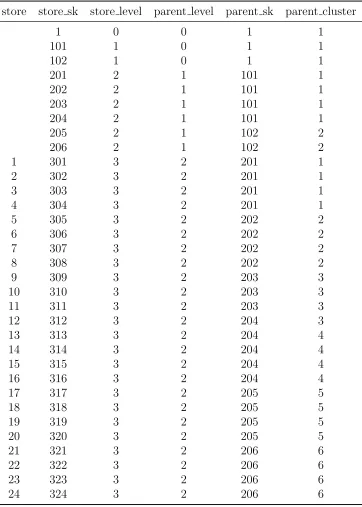
Table 4.1 Hierarchy Table . . . 88

Table 5.1 Set 1: Small-Sized Test Cases . . . 98

Table 5.2 Set 2: Medium-Sized Test Cases . . . 98

Table 5.3 Solution Status and Computational Time of the Direct Method . . 100

Table 5.4 Computational Time of the Naive Heuristic Method . . . 104

Table 5.5 Solution Status and Computational Time of the HD Heuristic Method107 Table 5.6 Percentage Difference of the Heuristic Methods/Time Limit = 60s 116 Table 5.7 Percentage Difference of the Heuristic Methods/Time Limit = 120s 116 Table 5.8 Percentage Difference of the Heuristic Methods/Time Limit = 180s 117 Table 5.9 Percentage Difference of the Direct Method/Time Limit = 1800s . 117 Table 5.10 Compare the Solution of the HD Heuristic Method with Optimal Solution . . . 122

Table 5.11 Extended Test Cases . . . 123

Table 5.12 Solution Status of the HD Heuristic Method . . . 125

(10)

LIST OF FIGURES

Figure 1.1 Pack Definition . . . 4

Figure 1.2 Merchandise Planning Procedure . . . 6

Figure 3.1 Three Types of Decisions . . . 53

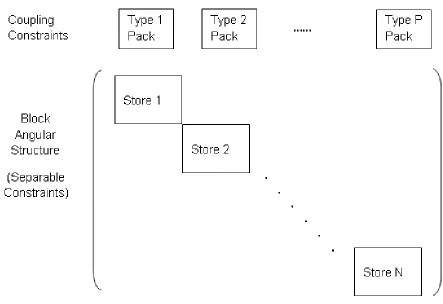
Figure 4.1 Block Angular Structure with Coupling Constraints . . . 61

Figure 4.2 Naive Heuristic Method . . . 63

Figure 4.3 Hierarchical Decomposition Heuristic Method . . . 69

Figure 4.4 Multi-Level Hierarchical Decomposition Heuristic Method . . . 78

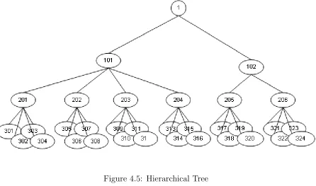
Figure 4.5 Hierarchical Tree . . . 89

Figure 5.1 An Example of the Generated Profiles . . . 94

Figure 5.2 Direct Method: BoxPlots of the Computational Time . . . 101

Figure 5.3 Direct Method: Computational Time vs Number of Stores . . . . 101

Figure 5.4 Direct Method: Histogram of the Computational Time when N = 8.102 Figure 5.5 Naive Heuristic Method: BoxPlots of the Computational Time . . 105

Figure 5.6 Naive Heuristic Method: Computational Time vs Number of Stores 105 Figure 5.7 HD Heuristic Method: BoxPlots of the Computational Time . . . 108

Figure 5.8 HD Heuristic Method: Computational Time vs Number of Stores 109 Figure 5.9 The Computational Time of the Scenarios with 64 and 88 Stores . 110 Figure 5.10 Percentage Difference of the Heuristic Methods/Time Limit = 60s. 113 Figure 5.11 Percentage Difference of the Heuristic Methods/Time Limit = 120s. 114 Figure 5.12 Percentage Difference of the Heuristic Methods/Time Limit = 180s. 114 Figure 5.13 Mean Percentage Difference of the Heuristic Methods/Time Limit = 60s. . . 118

Figure 5.14 Median Percentage Difference of the Heuristic Methods/Time Limit = 60s. . . 118

Figure 5.15 Mean Percentage Difference of the Heuristic Methods/Time Limit = 120s. . . 119

Figure 5.17 Mean Percentage Difference of the Heuristic Methods/Time Limit = 180s. . . 120

Figure 5.19 Mean Percentage Difference. . . 121

(11)

Figure 5.21 Box Plot of the Pct Diff of the HD Heuristic Method/Time Limit

= 60s. . . 124

Figure 5.22 Mean/Median of the Pct Diff of the HD Heuristic Method/Time Limit = 60s. . . 125

Figure A.1 A Sample of a Box Plot . . . 140

Figure B.1 Hierarchical Trees of the Test Scenarios . . . 142

(12)

Chapter 1 Introduction

Merchandise is commonly pre-packed for easy handling in a textile supply chain. The

merchandise at the lowest level of supply chain is named as thestock keeping unit (SKU).

A product line may consist of different SKUs differing in some attributes, such as the color

and size. Pre-packing lumps the merchandise into the packages of SKU combinations.

Such a package is treated as the basic flow unit in the supply chain planning and execution

cycle.

In this dissertation, we examine how the packing process affects the efficiency and

cost of a fashion appareli _{retail chain, which is named as the} _{pack optimization}

prob-lem. Mathematical formulations are provided for the problem. The complexity of the

problem is also studied. Exact and heuristic methods are proposed for solving the pack

optimization problem.

In this chapter, the background of the pack optimization problem is introduced in

Section 1.1. Section 1.2 presents the pack optimization problem and defines the scope as

i_{The emerging need of pack optimization originates from the fashion apparel industry, which is}

(13)

well as major assumptions of our study. Section 1.3 briefly introduces the models and

solution methods to be developed and implemented in our study. Finally, Section 1.4

(14)

1.1 Background

Before each selling seasonii _{begins, retailers often face a series of decision problems}

in-cluding ordering, allocation, and replenishment:

Ordering. Orders are placed by the distribution centers (DCs) to vendors.

Allocation. After the DCs receive the orders, they need to allocate the

merchan-dise to individual stores to fulfill the demands.

Replenishment. If the product is in low inventory or sold out in the middle of a

selling season, while more sales are coming, extra orders will be placed to stock up

the inventory.

The basic flow unit is a package. The advantage of this practice is that there are fewer

shipping units in the supply chain, which, as a consequence, increases the flow efficiency.

Section 1.1.1 provides the definition of inner and outer packs that will be deployed in the

pack optimization problem. Section 1.1.2 introduces the role of the packing decisions in

the supply chain workflow.

1.1.1 Pack Definition

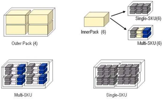
Two types of packs are commonly used: inner packs and outer packs, of which the

definitions are illustrated in Figure 1.1. An inner pack contains a specific number of

units of either identical SKUs (single-SKU inner pack) or different SKUs (multi-SKU

inner pack). In practice, a multi-SKU inner pack contains similar items differentiated

only by size. For example, an inner pack may contain 2 small, 3 medium and 1 large

SKUs. This practice is due to the large varieties of SKUs and small demand for each

(15)

SKU. An outer pack contains a specific number of identical inner packs. In Figure 1.1,

each block represents one SKU, the color of the block represents the size. As shown in

the figure, the inner pack containing blocks in the same color is a single-SKU inner pack,

while the one containing blocks in different colors is a multi-SKU inner pack. An outer

pack contain 4 identical inner packs in this case.

Figure 1.1: Pack Definition

Both outer packs and inner packs can be ordered by the DCs. An outer pack may

be sent directly to a store right after it arrives at the DC. It may also be opened at the

DC so that the resulting inner packs can be sent to various stores served by the DC.

Opening an outer pack provides more flexibility to meet the store demand at size-level

at an additional cost.

Sending a package to one store could possibly meet the demand of one item while over

(16)

because of the costs due to over-ordering or stockoutiii_{. Secondly, if a package needs to}

be opened at any point (e.g., DC, store), an opening cost applies. Therefore, the retailer

needs to determine a good packing strategy which should balance the flow efficiency

and demand satisfaction. The ultimate goal is to satisfy the store demand requirements

effectively, to enhance flow efficiency throughout the supply chain, and to minimize the

total involving cost. With all the considerations mentioned above, the development of

pack optimization becomes a challenging problem.

1.1.2 Packing Process in Supply Chain Management

A retailer buys goods or products in large quantities from vendors iv, and then sells to

the customers in small quantities. A large retailer may purchase tens of thousands of

products from thousands of vendors, it could be inefficient to ship each product directly

from each vendor to each store. Many large retailers run their own distribution networks,

while the small retailers may outsource this function to a dedicated logistics firm, who

coordinate the distribution of products for a number of retailers. In this dissertation, the

pack optimization problem provides solutions to large retailers mentioned above.

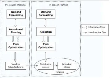
Figure 1.2 shows the decision process and information flow during the merchandise

planning horizon, and the merchandise flow within the supply chain. Most fashion

ap-parels are seasonal goods. This seasonality is not necessary to follow the actual season.

Instead, the seasonality is highly dependent on the product itself. For example, the

ac-tive selling season of a women’s trench coat can be early spring (January to March) or

iii_{Stockout is the situation where the demand or requirement for an item cannot be fulfilled from the}

available inventory. Stockout costs refers to the economic consequences of not being able to meet an interval or external demand from the current inventory. Such costs consist of internal costs (delays, labor time wastage, lost production, etc.) and external costs (loss of profit from lost sales, and loss of future profit). Stockout cost is also called shortages costs.

(17)

early Fall (August to October). In the fashion apparel industry, the lead time is usually

long. The retailers need to plan several months ahead for the coming season, which is

called thepre-season planning. The pre-season planning is normally 3 to 6 months earlier

than the active selling season of a product. Thein-season planning plans for the period

which begins when the retailers receive their order (at the DCs), and ends right before

the clearance.

Figure 1.2: Merchandise Planning Procedure

During the pre-season planning, retailers need to determine their orders to the vendor,

so as to fulfill the demand. The pack definitions are normally decided by retailers after

considering vendor constraints, if there is any. This decision on the retailer’s side is driven

(18)

predict weekly sales by store for a product (at the style color level). When doing the

assortment planningv_{, they need to distribute different sizes of a product to the stores.}

For example, a men’s Polo shirt in blue color may have sizes of ‘XS’,‘M’, ‘L’ and ‘XL’.

They need to decide exactly how many of each size to deliver to a particular store.

Once the DCs receive the packs from the vendor, the in-season period begins. During

the in-season planning, the packages have to be allocated to individual stores based on the

actual store demand of SKUs. In a scenario where the store demand cannot be fulfilled

in terms of packs, there are two choices. They can either open outer packs and then ship

some loose inner packs, or they can ship outer packs directly to individual stores. Either

way has cost implications. Different methods will affect the number of SKUs received at

individual stores. The packing exercise at this point can be focused on minimizing the

overall cost, including handling cost, opening pack cost and mismatch penalty cost.

In the ideal scenario where the forecasted demand coincides with the actual demand,

the packing decision can be made during the pre-season planning horizon, and the same

decision can be implemented for allocation purpose. However, this is usually not the

case in reality. The actual demand may vary significantly from the forecasted demand,

mainly due to the uncertainty in forecasting and the time difference between ordering and

sales. Ordering to vendors may precede store allocations and sales by several months,

especially for the global business. Events, unaccounted for by the forecasting model,

could occur and affect the accuracy of forecast, such as an economic downturn, a local

festival, etc.. Forecasting accuracy increases as time gets closer to the selling season of

the product. Therefore, at the time of allocating the packs from DC to individual stores,

v_{Assortment planning breaks the Merchandise Plan down to the components that enable the planner}

(19)

better forecasts might be available and allocation decisions should be adjusted.

To sum up, in the supply chain, there are two major decisions that are impacted by

the packing process. The first one is the configuration of purchasing orders in terms of the

outer and inner packs, which is based on the demand forecast made several months before

the SKUs reaching the store. The second decision is the allocation of packs to stores to

reduce the opening costs of outer packs and demand mismatches, which is based on the

demand forecast made a couple of days before the SKUs reaching the store. Therefore,

(20)

1.2 Problem Statement

In the literature, the white paper written by Inderlal and Divyanshu [44] is the first

one to introduce the pack optimization problem for the fashion retail industry. The

white paper states that “An efficient pre-pack decision-making process involves taking

multiple decisions throughout the supply chain management cycle, starting right from the

demand forecast to initial planned allocation during assortment planning, purchase order

generation, as well as allocation performed at the distribution centers”. In other words, a

successful pack optimization solution requires robust demand forecasting as well as good

assortment planning. Inderlal and Divyanshu suggested a workflow for determining the

optimal pre-pack solution. The flow tells when and how to define a pre-pack. They also

presented mathematical models for the problem but did not give any solution methods.

Inderlal and Divyanshu’s white paper, which is mainly for marketing purpose, is an

article devoted to promoting the pack optimization problem rather than building up the

theoretical foundation. Although some simple mathematical programming models are

presented in the paper, which is also the only paper we can find in the literature, no

solution approach has been proposed. There are some research conducted in a close

related field of assortment planning [52, 45]. However, the research on pack optimization

has never been formally introduced nor mathematically formalized in the academic field.

As shown in Figure 1.2, solving the pack optimization problem requires information

from assortment planning (pre-season) and allocation (in-season). An optimal packing

solution outputs the pack composition, which optimally matches the store-level demand

for the merchandise to the pack-level supply of merchandise. In addition, it also

commu-nicates with other modules in the supply chain, to increase the supply chain efficiency

(21)

implementation of pack optimization may lead to great economic benefits.

In the fashion apparel retail industry, the SKU combination in a pack is normally

defined by the vendor. However, sometimes it is up to the retailer, such as Wal-Mart,

to decide the pack definition. In other words, the ones in the leader’s position may

give the pack definition. There are two versions of the pack definition. One is to take

the existing pack definition from retailers directly. The other is to make it as decision

variables of the pack optimization problem. The latter scenario extends the problem

to a “pack recommendation problem”. In our dissertation, we study the problems with

existing pack definitions, and multi-SKUs are allowed in each pack.

The scope of the dissertation is to make optimal packing decisions for retailers. The

goal is to minimize the sum of the costs over the DC and individual stores, including the

handling cost, opening pack cost and mismatch penalty cost. The following assumptions

are made for this study:

1. There is one DC which serves all stores. In reality, DC may serve several stores and

a store may be served by two or more DCs. To simplify the problem, it is assumed

there is only one DC and all stores get supplies from the single DC.

2. The DC cannot hold inventory. In other words, all packs that get into the DC

should be allocated to individual stores.

3. No inner packs can be opened at the DC.

4. The demand for the entire planning season is known. As discussed in Section 1.1.2,

the accuracy of demand forecast changes as time goes by. Probabilistic demand

might be better in presenting the reality. To simplify the scenario, a deterministic

(22)

forecast, made at any time, is the same as the actual demand, in other words, it

should not change across the planning horizon.

5. One order is placed per planning season, which means that no backorder and no

replenishment can happen. The assumption could be reasonable for the fashion

industry, where the lead time can be up to 6 months.

6. All the costs involved are linear. In the packing process, a series of costs incur as

the flow goes through the supply chain. Our study is to help the retailers make

the best packing decisions. Therefore, we will focus on the costs at the DCs and

individual stores, which includes the handling cost and opening pack cost. Since the

pack configuration affects the demand fill rate vi _{and stockout rate}vii_{, a mismatch}

penalty cost is also included in the cost function.

Although mismatches are allowed, each store may have a tolerance interval for the

shipment. For each SKU, there exist lower and upper limits for the number of items

received by each store. In particular, it is required that the number of items to be

received by each store be more than its corresponding lower limit and capped by its

corresponding upper limit.

To sum up, the scope of the dissertation is to make optimal packing decisions for

retailers. The goal is to minimize the sum of the costs over the DC and individual stores,

including the handling cost, opening pack cost and mismatch penalty cost. The following

assumptions are made for this study:

1. There is one DC which serves all stores.

vi_{Percentage of customer or consumption orders satisfied from stock at end. It is a measure of an}

inventory’s ability to meet demand.

vii_{Percentage of customer or consumption orders unsatisfied due to stockout. It is a measure of the}

(23)

2. The DC cannot hold inventory.

3. No inner packs can be opened at the DC.

4. The demand for the entire planning season is known.

5. One order is placed per planning season, which means that no backorder and no

replenishment can happen.

6. All the involving costs are linear.

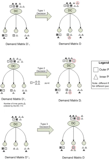
To provide a complete solution to the pack optimization problem, we need to determine

the number and type of outer and inner packs that should be ordered by the DC. We

also need to decide the number of outer packs to be opened at the DC before allocating

to individual stores. Finally, we need to know the numbers of outer and inner packs to

(24)

1.3 Models and Solutions Methods

The pack optimization problem will be formulated as an integer programming problem

(IP) in Chapter 3. It is a straight-forward way of interpreting the problem

mathemat-ically. The resulting IP model can be solved by using some commercial softwares, for

example, SAS/OR, CPLEX, etc., given that the time and computational resources are

sufficient. However, it may not be an efficient way for solving practical problems.

A dynamic programming (DP) model is presented in Chapter 3 to help understand

the complexity of the problem. A DP-based algorithm is also developed. However, the

DP-based algorithm is not an efficient approach for solving large scale pack optimization

problems. Nevertheless, the process of building a DP model and developing a DP-based

approach for the problem may reveal some hidden properties of the problem.

Two heuristic methods: a naive heuristic method and a hierarchical decomposition

(HD) heuristic method, are developed based on some special structures of the problem.

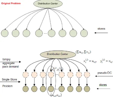
The naive heuristic method treats each individual store separately and breaks the original

problem to multiple “single-store” problems. After solving each of the “single-store”

problem, the solutions are aggregated together to form a solution of the original problem.

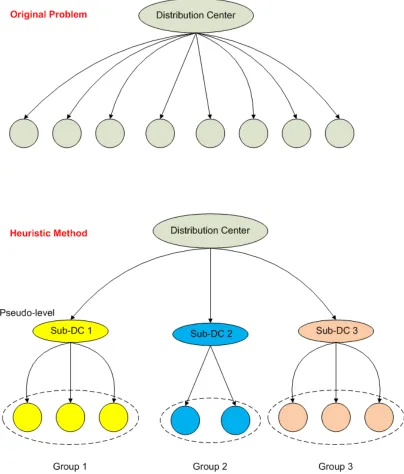
It is a quick and dirty approach. In the HD heuristic method, a hierarchy tree is created

and the original problem is decomposed into several small size problems at different

levels of the tree. The computational efforts is eased through the decomposition. These

subproblems are solved from top to down. Computational experiments indicate that this

(25)

1.4 Outline

This dissertation is organized as follows: Chapter 1 provides a brief introduction to the

pack optimization problem, including the background, problem statement, related issues,

as well as the proposed models and solution approaches. Chapter 2 is a literature review

on the related knapsack problem and frequently used solution approaches including the

dynamic programming approach and Lagrangian and surrogate methods. In Chapter 3,

an integer programming model of the pack optimization problem is built. The size of the

model is analyzed. A dynamic programming model is also presented, which deals with

a special case of the pack optimization problem with an additional assumption that no

mismatch is allowed. In Chapter 4, two heuristic methods are proposed. Computational

experience and results are reported in Chapter 5. The limitation of the direct method

(solving the IP model directly) is shown to be the most time-consuming. The naive

heuristic method is shown to be most time efficient, while the hierarchical decomposition

heuristic method is efficient in terms of the computational time and effective in terms of

the solution quality. Pros and cons of each method are summarized. Improvements on

the heuristic methods are also recommended. Chapter 6 gives some concluding remarks

(26)

Chapter 2 Literature Review

The pack optimization problem is new to academic, there is no paper directly discussing

the pack optimization problem in the literature. However, it is related to some existing

problems, of which the most widely studied one is the knapsack problem because of

its wide applications. This chapter reviews the literature on the related problems and

solution methods.

In Section 2.1, we conduct a review over the multidimensional knapsack problem and

multiple knapsack problem, since both problems are closely related to the pack

opti-mization problem. The pack optiopti-mization problem is formulated as an integer problem

in Chapter 3. Therefore, in Section 2.2, we review some solution approaches for

solv-ing integer programmsolv-ing problems includsolv-ing dynamic programmsolv-ing and Lagrangian and

(27)

2.1 Knapsack Problem

Suppose that someone plans to climb a mountain. He can choose among various types

of food to put into his knapsack. The goal is to maximize the nutrition he gets without

exceeding the knapsack capacity (for example, weight). This type of problem is called a

knapsack problem. Number these items from 1 to n. Define the following notations:

pj: the nutrition of item j, for j = 1,· · · , n.

wj: the weight of item j, forj = 1,· · · , n.

b: the knapsack capacity, which is the maximum weight that the knapsack can hold.

xj: the number of item j to be selected, for j = 1,· · · , n.

Then the knapsack problem can be mathematically formulated as follows:

maximize Pn

j=1pjxj (2.1)

subject to Pn

j=1wjxj ≤b, (2.2)

x∈Zn

+. (2.3)

Two types of the knapsack problem are normally considered. One is the 0-1 knapsack

problem withxj = 0 or 1. The other is the bounded knapsack problem where the number

of each item j has an upper bound uj, i.e., 0≤xj ≤uj and xj is an integer.

The special structure of the knapsack problem and its generalizations have attracted

researchers to tackle this problem using various mathematical programming techniques.

Progress has been made over the years and formed a rich literature. Various approaches

(28)

Kellerer, Pferschy and Pisinger [49] provided comprehensive surveys on the knapsack

problem.

There are many variants and extensions of the knapsack problem. Lin [55] provided a

bibliographical survey on some well-known extensions of the knapsack problem. The most

frequently studied generalizations include themultidimensional knapsack problem,

multi-ple knapsack problem,multiple choice knapsack problem andquadratic knapsack problem.

For a comprehensive list of the generalizations of the knapsack problem, one can refer

to Chapter 13 of the book of Kellerer, Pferschy and Pisinger [49]. The multidimensional

knapsack problem (d-KPi_{) is a knapsack problem with multiple resource constraints. The}

goal is to determine a subset of the items such that the total profit is maximized and all

resource constraints are satisfied. Themultiple knapsack problem (MKP) is another

vari-ation of the standard knapsack problem. It extends the original knapsack problem from

a single knapsack tom knapsacks with (possibly) different capacities [49]. The objective is to assign each item to at most one of the knapsacks so as to maximize the total profit

without violating any of the constraints. Themultiple choice knapsack problem (MCKP)

arises from the following case: the items are partitioned into several mutually exclusive

sets, and at most one item per set can be selected. As a result, one more constraint

is imposed for each set in addition to the single resource constraint. Another variant

appears if an item has a corresponding profit, and an additional profit is redeemed if the

item is selected with another item. The objective is still to select among the items so

that the total profit is maximized, and the capacity constraint is not violated. This is

the so-called quadratic knapsack problem (QKP).

i_{There are several short forms for the multidimensional knapsack problem in the literature, for}

(29)

As discussed in Section 1.3, both the d-KP and MKP are subproblems of the pack

optimization problem. the solution methods and algorithms for the d-KP and MKP are

reviewed in Section 2.2.1 and Section 2.2.2, respectively.

2.1.1 Multidimensional Knapsack Problem

The multidimensional knapsack problem (d-KP) is a knapsack problem with multiple

resource constraints. It can be mathematically formulated as

maximize Pn

j=1pjxj (2.4)

subject to Pn

j=1wijxj ≤bi, i= 1,· · · , m, (2.5)

x∈Zn

+, (2.6)

where wij is the amount of resource i consumed by item j, and bi is the maximum

capacity of resource i. The d-KP has received attention for its applications, including the capital budgeting problem (Lorie and Savage [56] and Weingartner [84]), cutting

stock problem (Gilmore and Gomory [30]), project selection problem (Petersen [69]),

cargo loading problem (Shih [76]), resource allocation problem (Gavish and Pirkul [25])

and many others. Since the 0-1 knapsack is well known to be NP-hard (Martello and Toth

[64]), it follows that the d-KP is NP-hard. Due to its NP-complexity, most of the work

in the literature are focusing on finding approximation algorithms or heuristic methods

to solve the problem. Exact solution approaches, therefore, receive less attention. And

not to be surprised, most exact methods are reported to be efficient only for small size

problems.

The basic idea in most solution approaches, either exact or approximate, is to transfer

(30)

algorithms. The techniques of Lagrangian relaxation and surrogate relaxation therefore

have been widely used. The multiple resource constraints of d-KP can be aggregated

to a single constraint through surrogate relaxation. It can also be decomposed into

several single-constraint knapsack problems by dualizing the resource constraints using

Lagrangian relaxation. The theoretical relation of Lagrangian relaxation, surrogate

re-laxation and composite rere-laxation (i.e., combined Lagrangian and surrogate rere-laxations)

for the 0-1 d-KP have been studied by Gavish and Pirkul [26]. They also provided a

detailed study of the computation of the multipliers concentrating on the d-KP.

Heuristic Solution Approaches

A major part of the research on heuristics for d-KP deals with the utilization of

relax-ations. LP relaxation is the most straightforward relaxation, which simply removes the

integer constraints, or replaces them by linear constraints (e.g., replace binary constraint

for variable xwith 0 ≤x≤1). Lagrangian relaxation and surrogate relaxation also play important roles in providing bounds for approximate solutions.

Senju and Toyoda [75] first proposed a dual gradient method to find approximate

solutions of the 0-1 d-KP. The method starts with all variables being set to one. It

then follows an effective gradient path which searches for a feasible solution by setting

one variable at a time to zero according to increasing reward to weight ratios until the

feasibility is reached. In contrast, the KOCH method presented by Kochenberge, McCarl

and Wyman [50] builds up a solution by assigning a value of one to one variable at a time

until it reaches infeasibility. Magazine and Oguz [59] proposed an LP based heuristic

method called Multi-Knap. Their method combines the idea of Senju-Toyoda’s [75]

heuristic method with Everret’s [20] generalized Lagrange multipliers approach for solving

(31)

from the LP relaxation directly without any additional effort. The algorithm is compared

with Senju-Toyoda’s [75] method and KOCH [50]. KOCH starts with a feasible solution

and stops when it reaches infeasibility, while the other two starts with an infeasible

solution and try to reach feasibility. KOCH performs better when the constraints get

tighter, in opposite to the other two. Senju-Toyoda’s method is better when the constraint

is loose, in terms of the quality of the solution. For large size problems, Multi-Knap

almost matches KOCH in performance, and reduces the computational time significantly.

In contrast to the dual gradient method, Toyoda [80] developed a primal gradient

method, which is an enhanced version of KOCH [50]. By incorporating the primal gradient

method of Toyoda [80] and the greedy method for the solution of standard knapsack

problem, Loulou and Michaelides [57] developed a greedy-like heuristic method. The

greedy-like heuristic method expands the feasible solution by including the variable with

the maximum utility instead of the effective gradient as in Toyoda. The

pseudo-utility of a variable represents the profit per unit of resource consumed by this variable.

Computational results show that the greedy-like heuristic method performs better than

the primal dual method in terms of solution quality. However, the CPU time consumed

is slightly higher.

Fr´eville and Plateau [23] proposed aLagrangian and surrogate relaxation based heuris-tic algorithm to solve the d-KP. It was the first algorithm using the idea of perturbing

the solutions to surrogate relaxations and updating the multipliers to obtain good

feasi-ble solutions. Fr´eville and Plateau constructed three sets of surrogate multipliers: from the Lagrangian dual, from the surrogate dual, and from a structural multiplier. Two

linear time heuristics AGNES1 and AGNES2 were proposed to solve the surrogate

(32)

con-junction of tests applied to Lagrangian and surrogate relaxations of the original problem.

Computational results have shown encouraging performance of the heuristic algorithm.

Later Fr´eville and Plateau improved the heuristic approach by introducing an efficient subgradient method [24] which effectively controls the step-size. As a result, both the

lower and upper bounds of the d-KP are sharpened. In addition, a new reduction scheme

was also introduced. Fr´eville and Plateau’s improved heuristic method that can serve as an efficient preprocessing procedure for solving large-size d-KP.

Pirkul [70] proposed a surrogate duality approach for the d-KP based on the

opti-mality theory reported by Gavish and Pirkul [26]. Pirkul’s method first solves a series

of LP relaxed standard KP problems. Each has the constraint corresponding to one of

the resource constraint in the d-KP. The solution associated with the minimum objective

value is chosen as the initial set of surrogate multipliers. The set of surrogate

multipli-ers is improved by taking into consideration the most violated resource constraint until

all resource constraints are satisfied. An approximate solution to the d-KP is obtained

by solving the standard knapsack problem, which is resulted from the set of surrogate

constraints based on the ordering of the return to resource consumption ratios.

Com-putational results show that the proposed surrogate dual approach performs better than

Loulou and Michaelides’ [57] both in computational time and solution quality.

Volgenant and Zoon [82] presented a method called K2UB which improved the

heuris-tic method presented by Magazine and Oguz [59]. Instead of computing the values of

multipliers one per iteration (as in [59]), it computes k values simultaneously in one

iteration. It also provides an improved upper bound. Both methods are programmed

in Pascal. In general, the method K2UB obtains better solution than Multi-Knap and

consumes a modest amount of extra computing time.

(33)

can be realized with Lagrangian and surrogate relaxations. They showed that the

im-provement of the bound cannot exceed the largest coefficient in the objective function.

Moreover, it cannot exceed one-half of the optimal objective-function value of linear

re-laxation. In particular, it implies that for a problem where all coefficients in the objective

function are 1, the bound derived by the Lagrangian and surrogate relaxation cannot be

better than the one by simply rounding the solution of linear relaxation.

Osorio, Glover and Hammer [68] focused on the generation of logic cuts by using

surrogate analysis and constraint pairing. They allow variables to be fixed at zero based

on the reduced costs associated with the LP relaxation. The rest are then put into two

groups: those tend to zero and those tend to one. Computational results show that

their method uses less number of nodes in the search tree than those leading commercial

softwares including CPLEX. They also reported that when augmented with the proposed

approach, CPLEX performed much better on average.

Bertsimas and Demir [8] presented an approximate dynamic programming (ADP)

approach for the d-KP. They approximated the value function using two methods. The

first method is to use parametric and nonparametric methods. The second method is

to use a base-heuristic. Their new heuristic approach adaptively rounds the solution

of the LP relaxation problem. It is reported to produce high quality solutions fast

and robustly, even faster than CPLEX. The ADP approach using the new heuristic

algorithm outperforms other heuristics such as the genetic algorithms. The ADP based

on parametric and nonparametric is not so competitive.

Instead of using a single technique to develop the heuristic approach, people also

started to exploit the features of different heuristics and try to combine the good features

of different heuristics together. This leads to some hybrid algorithms. The resulting

(34)

But through the clever combination of different heuristics, it can obtain very good solution

values for many classes of the problem. The four phase heuristic AGNES by Fr´eville and Plateau [24] is a typical example of the hybrid algorithm.

The heuristic method proposed by Lee and Guignard [53] is also a hybrid method. It

incorporates the modified version of the primal gradient method of Toyoda [80] and the

complement operations of the Balas and Martin algorithm [2]. Computational results

show that their procedure generates better results than Toyoda [80] and Magazine and

Oguz [59], and consumes less time than the latter but not the former. It is also faster

than Balas and Martin algorithm [2], but obtains a little worse solution values. A recent

paper of Thiongane, Nagih and Plateau [78] is a successful application of the hybrid

algorithm.

Due to the complexity of the problem, meta-heuristics have been applied and tested

in the field of the d-KP. Battiti and Tecchiolli [6] marked the importance of the d-KP

as a benchmark problem in their study on reactive tabu search. We will not give a

detail review on this subject since it is not the major view of our study. Here, we only

mention some surveys. Hanafi, Fr´eville and El Abdellaoui [38] provided a good survey on existing contributions in this field. Chu and Beasley [10] not only proposed a new

genetic algorithm for solving the d-KP, but also presented a comprehensive survey of

existing heuristics. For an overview of tabu search approaches, one can refer to Hanafi

and Fr´eville [37].

Exact Solution Approaches

The development of exact algorithms for solving the KP began in the 1960s. The

d-KP is closely related to the general IP problems with the restrictions that all knapsack

(35)

the literature, the classical branch-and-bound algorithms for general integer programming

is frequently applied for calculating the optimal solution of the d-KP. Some attempts to

tackle the problem were also made by dynamic programming.

Gilmore and Gomory [32] are among the first to develop an exact approach with a

modified dynamic programming algorithm. The algorithm is based on a major

character-istic of one dimensional cutting stock problem, i.e.,F(x1+x2)≥F(x1) +F(x2). Where

x1 andx2 are the length of each item, and F(x) is the knapsack objective function value

when the length of the item is x. This characteristic is extended into two dimensional problem and used in the dynamic programming forward recursion equation. However,

the characteristic exists only for guillotine cutsii_{. The inequality is not necessary to hold}

for non-guillotine cuts.

Weingartner and Ness [85] proposed a dual approach applied within a dynamic

pro-gramming framework to find an exact solution. In the complement problem, all items

are included at the beginning. During the dynamic programming iterations, it

elimi-nates one variable at a time, from the existing solution, until a feasible solution is found.

Nemhauser and Ullmann [67] extended the work of Weingartner and Ness [85]. For more

literature on improving the dynamic programming algorithm, one can refer to Pisinger

[72] and Balev et al. [4].

Balas [3] presented a branch-and-bound approach for solving general integer

program-ming problems. In his approach, all the variables start at zero and increase to one based

on a systematic pseudo-dual algorithm. The earliest paper containing a

branch-and-bound algorithm especially for the d-KP was given by Thesen [77].

ii_{A cut is called a}_{guillotine cut} _{if it breaks a connected area into at least two pieces, otherwise it is}

(36)

Shih [76] designed the first linear programming based branch-and-bound approach

which takes advantage of the special structure of the 0-1 d-KP. It treats the original

problem as m single-constraint binary knapsack problems. Each problem has the same objective function and one of the resource constraints of the original problem.

Compu-tational results show that Shih’s method outperforms Balas’ additive algorithm [3] and

the improved Balas algorithm (Kuester and Mize [51]) in terms of the solution time and

the number of iterations.

2.1.2 Multiple Knapsack Problem

Themultiple knapsack problem (MKP) is another generalization of the standard knapsack

problem. It arises when m knapsacks of possibly different capacities ci (i = 1,· · · , m)

are available. Define the following notations:

pij: the profit of putting item j in knapsack i, for j = 1,· · · , n, i= 1,· · · , m.

wij: the resource consumed by putting item j in knapsack i, for j = 1,· · · , n,

i= 1,· · · , m.

xij: the number of item j selected to put into knapsack i, for j = 1,· · · , n, i =

1,· · ·, m.

The MKP can be mathematically formulated as

maximize Pm

i=1

Pn

j=1pijxij (2.7)

subject to Pn

j=1wijxij ≤ci, i= 1,· · · , m, (2.8)

(37)

A classical application of the MKP can be found in the cargo loading problem (Eilon and

Christofides [18]). The same as in the d-KP, the branch-and-bound scheme is frequently

used for solving the MKP. However, dynamic programming algorithms rarely appear in

the literature for this case. The reason is that the MKP does not admit a fully polynomial

time algorithm scheme (FPTAS) unless P = N P [12, 14]. Lagrangian relaxation and surrogate relaxation are among the most popular techniques for providing good lower

and upper bounds in branch-and-bound schemes.

Branch-and-Bound Scheme and Lagrangian/Surrogate Relaxation

Several Branch-and-Bound algorithms for the MKP have been presented. For example,

the algorithms presented by Neebe and Dannenbring [66] and Eilon and Christofides [18]

are designed for problems with many knapsacks and relatively few items. The algorithms

presented by Hung and Fisk [42], Martello and Toth [62, 63] and Pisinger [73] are best

fit for problems with a large number of items and few knapsacks.

Hung and Fisk [42] proposed a branch-and-bound procedure. Various bounding

tech-niques based on Lagrangian and surrogate relaxations have been investigated.

Com-putational results show that the incorporation of surrogate constraints is more efficient

for smaller size problems, while the incorporation of the Lagrangian relaxation is more

efficient for larger size problems.

Martello and Toth [62] presented a different branch-and-bound scheme utilizing the

Lagrangian relaxation technique. Algorithms are developed by using two different

branch-ing strategies and boundbranch-ing procedures, namely MTL and MTLS. The proposed

algo-rithm is compared with Hung and Fisk’s algoalgo-rithm [42]. They refer to HFS for Hung

and Fisk’s algorithm if it is based on surrogate relaxation, HFL if based on Lagrangian

(38)

results show that MTL is better than MTLS when m= 2, and worse when m >2. HFS is better than HFLS when m = 2, and worse when m > 2. Later Martello and Toth [63] improved the branch-and-bound scheme and presented a Bound and Bound (called

MTM) framework. The MTM framework has the advantage that it can avoid updating

all variables. The Bound and Bound algorithm based on the MTM framework is

com-pared with Hung and Fisk’s algorithm and MT (MTL and MTLS [62]). Computational

results show that it outperforms the other two.

Pisinger [73] presented a MulKnap algorithm based on the MTM framework. The

framework has been improved in several aspects. First of all, lower bounds are derived

by solving a series of subset-sum problems. The subset-sum problems are also used for

tightening the capacity constraints of each knapsack. Secondly, better upper bounds are

obtained through surrogate relaxation. DP is used to solve each individual subset-sum

problem. The algorithm is the first one designed for solving large size problems with the

number of knapsacks up to n = 100000.

A recent paper in the field is presented by Yamada and Takeoka [86]. Their method

obtains upper bounds using Lagrangian relaxation and lower bounds using a greedy

heuristic approach. A branch-and-bound algorithm is also presented. At each terminal

subproblem, it solves the MKP exactly by invoking the MulKnap code written by Pisinger

[73].

Approximation Algorithms

The building of polynomial time approximation scheme only starts recently. Caprara,

Kellerer and Pferschy [12, 13] presented a polynomial time approximation scheme (PTAS)

for the multiple subset sum problem. It described a 2/3-approximation algorithm. After

(39)

Khanna [14] generalized the results and presented a PTAS for the MKP with different

capacities. They also presented a guessing strategy which can provide in polynomial

time almost all the items that are packed by an optimal solution. For the MKP with

assignment restrictions, Dawande et al. [15] showed that simple greedy approaches yield

1/3-approximation algorithms for the objective of maximizing assigned weight. The

dominant property is also exploited to reduce the search space (see Balachandar and

Kannan [1]). Wang and Xing [83] utilized the dominant property and presented a

succes-sive approximation algorithm that packs the knapsacks in nondecreasing order of their

capacities. It analyzes the algorithm for solving the 2 and 3 knapsack problems by a

worst-case analysis and provides error bounds. The error bounds of their approximation

(40)

2.2 Models and Solution Methods

In this section, we review the approaches we intend to apply for solving the pack

opti-mization problem. Dynamic programming has been used to find exact solutions of the

knapsack problems. Despite the fact that most of the time it fails to perform efficiently

in solving large size problems, it is still a popular method. The main reason is that the

algorithm identifies the basic components of the original problem, which can help people

understand the details of the problem.

As regard to the heuristic methods, most papers in the literature for solving the d-KP

and MKP, tend to relax the original problem, or decompose the original problem into

subproblems. Each subproblem is a single-constraint knapsack problem. As a result,

La-grangian and surrogate methods have been frequently used. The combination of the two

methods is the so-called composite relaxation (i.e., combination of Lagrangian relaxation

and surrogate relaxation) or composite dual (i.e., combination of Lagrangian dual and

surrogate dual). It is introduced by Greenberg and Pierskalla [35] in 1970. An

intro-duction and brief review of dynamic programming, Lagrangian methods and surrogate

methods is presented in the following three subsections.

2.2.1 Dynamic Programming Approach

Dynamic programming (DP) is both a mathematical optimization model and a computer

programming method. In both contexts, it refers to simplifying a complicated problem

by breaking it down into simpler subproblems in a recursive manner. The technique of

DP is introduced by Bellman [7]. If subproblems can be nested recursively inside larger

problems, so that DP methods are applicable, then there is a relation between the value

(41)

relationship is called the Bellman equation.

There are a number of characteristics that are common to all dynamic programming

problems. They are listed as follows:

1. The problem can be divided into stages with a decision required at each stage.

2. Each stage has a number of states associated with it.

3. The decision at one stage transforms one state into a state in the next stage.

4. Given the current state, the optimal decision for each of the remaining states does

not depend on the previous states or decisions.

5. There exists a recursive relationship that identifies the optimal decision for stage

j, given that stage j+ 1 has already been solved.

6. The final stage must be solvable by itself.

The last two properties are tied up in the recursive relationship given above. The major

skill in dynamic programming, and the art involved, is to take a problem and determine

the stages and states so that all of the above characteristics hold.

The knapsack problem has the property of an optimal structure as described above.

Assume that the optimal solution of the knapsack problem has already been computed

for a subset of the items, and part of the knapsack capacity has been used. Then we

add one item to this subset and check whether the optimal solution needs to be changed

for the enlarged subset. This check can be done very easily by using the solutions of

the knapsack problems with a smaller capacity. To preserve this advantage we have to

compute the possible changes of the optimal solutions for all possible capacities. This

procedure of adding an item is iterated until finally all items are considered. Then an

(42)

Consider the function

f(n, b) = max

( _n X

j=1

pjxj| n

X

j=1

wjxj ≤b, xj ∈ {0,1}, j = 1,· · ·, n

)

, (2.10)

which represents a 0-1 knapsack problem with f(n, b) being the optimal value of the problem. The optimal value can be found using the recursion

f(k, g) = max{f(k−1, g), pk+f(k−1, g−wk)}, (2.11)

fork= 1,· · · , nandwk ≤g ≤b. The recursion is initialized byf(0, g) = 0 for 0 ≤g ≤b.

Gilmore and Gomory developed the first DP model for the KP and two dimensional

KP in in 1966 [32] . Toth presented a DP-based approach for the KP in [79] and reported

numerical experiments with limited success. More recently, Pisinger [71] proposed a DP

algorithm for the KP. It constructs a core problem of minimal size, which can minimize the

sorting and reduction efforts. Hybrid methods, combining DP and implicit enumeration,

were developed for the KP. The first approach was published by Plateau and Elkihel [74].

An approach proposed later by Martello, Pisinger and Toth [61], called combo algorithm,

is able to solve very large instances with 10000 variables in one second. There is basically

no difference in the solution time of solving “easy” and “hard” instances.

Marsten and Morin [60] proposed the first hybrid method for the d-KP, which

com-bines the heuristic algorithms, DP method and branch-and-bound approaches. More

sophisticated methods such as a successive sublimation procedure can be found in [43].

Bertsimas and Demir [8] presented an approximate dynamic programming (ADP)

ap-proach for the d-KP and reported fairly good computational results. Balev et al. [4]

(43)

shows that their reduction procedure can improve the CPU time of leading commercial

softwares such as CPLEX. The MKP has been proven to be strongly NP-hard even when

m = 2 (only two knapsacks). Therefore, very few literature can be found to apply DP for solving the MKP.

2.2.2 Lagrangian Method

The introduction of Lagrangian relaxation methods simplifies many hard IP problems.

These hard IP problems can be viewed as an easy problem with some complication caused

by a relatively small set of side constraints. The idea is to dualize the side constraints

using Lagrangian multipliers such that the resulting problem is relatively easy to solve.

The optimal value of the Lagrangian relaxed problem provides an upper bound (for

maximization problem) for the optimal value of the original problem. Consider an integer

programming P in general form

maximize Pn

j=1cjxj (2.12)

subject to P

j=1aijxj ≤bi, i= 1,· · ·, m, (2.13)

x∈Z₊n. (2.14)

The Lagrangian relaxed problem L(P, λ) can be written as

maximize Pn

j=1cjxj−

Pm

i=1λi

P

j=1aijxj −bi

(2.15)

x∈Zn

+, (2.16)

where λ = (λ1,· · · , λm) is a vector of nonnegative Lagrangian multipliers. The relaxed

(44)

objective function (2.15). Since all feasible solution for P is also feasible for L(P, λ), it naturally leads to the fact that z∗(L(P, λ)) ≥ z∗(P), where z∗ denotes the optimal solution of the problem.

In a branch-and-bound algorithm, we would like to achieve the tightest upper bound

for P. The goal can be achieved by finding a vector of Lagrangian multipliers such that problem L(P, λ) is minimized, namely, the Lagrangian dual problem LD(P) where

z(LD(P)) = min

λ≥0 z(L(P, λ)). (2.17)

Lagrangian decomposition is also a technique of great interests. The idea is to split

the problem into a number of independent problems which can be solved efficiently.

By copying variables and linking them to original variables, as well as a Lagrangian

relaxation, one hopes to be able to decompose the resulting Lagrangian relaxed problem

into several independent subproblems. By introducing copy variables xi

j to the problem

P, where i = 2,· · · , m, for each variable xj and link them to x1j, the following model

applies:

maximize

n

X

j=1

cjxij (2.18)

subject to

n

X

j=1

aijxij ≤bi, i= 1,· · ·, m, (2.19)

x1_j =xi_j, i= 2,· · ·, m, j = 1,· · · , n, (2.20)

(45)

Taking Lagrangian relaxation of constraint (2.20), it becomes

maximize

n

X

j=1

cjxij − m X i=2 λi n X j=1

x1_j −xi_j (2.22)

=

n

X

j

cj− m

X

i=2

λi

! x1_j +

m X i=2 λi n X j=1

xi_j (2.23)

subject to X

j=1

aijxij ≤bi, i= 1,· · · , m, (2.24)

x∈Z₊mn. (2.25)

The problem can now be decomposed into m independent single-constraint IP problems

maximize zi =Pn_j₌₁cijxij (2.26)

subject to Pn

j=1aijx

i

j ≤bi, (2.27)

x∈Zmn

+ , (2.28)

where c1

j = cj −Pm_k₌₂λk and cij =λi for i = 2,· · · , m. The overall solution is found as

z =Pm

i=1zi.

The Lagrangian relaxation and decomposition techniques have been intensively

stud-ied during the past five decades. It plays a fundamental role in discrete optimization

problems and has been widely used in solving many classical problems. For example, the

generalized Lagrange multipliers approach for solving resource allocation problem in [20],

the well-known column generation techniques applied in cutting stock problem in [30], the

highly successful Lagrangian-based algorithm for the traveling salesman problem (TSP)

in [39, 40], the multiplier adjustment method based-algorithm for solving generalized

(46)

improv-ing sequences for solvimprov-ing generalized assignment problem and multiple-choice knapsack

problem in [5], Lagrangian relaxation combined with branch-and-bound for solving

lot-sizing problems in [16]. More applications can be found in the literature. Theoretical

development in the Lagrangian approaches can be found in [29, 9, 36, 87].

A classical reference for the application of the Lagrangian relaxation methods in

solving the IP problems is given by Fisher [21]. It gives a review and a framework of

the approach. Fisher proposed five issues which arise from applications. First of all,

how to find the appropriate values for multipliers? Secondly, is it possible to get a

relaxed problem whose objective value is close to or equal to the optimal value of original

problem? This problem is closely related to the first one. Thirdly, which constraints

to dualize. Fourthly, how to achieve primal feasibility from the Lagrangian relaxations?

Finally, how to integrate the bound obtained from Lagrangian relaxation in a

branch-and-bound method? Each of the issues is discussed below.

Many efforts have been spent on finding the values for the multipliers. For the

non-differentiable case, three approaches are discussed. The first approach is the subgradient

method. The second one is the simplex-based method with column generation. The third

one is the multiplier adjustment method. The subgradient method is the most widely

used one. Held et al. [41] discussed the computational performance and theoretical

con-vergence properties of the subgradient method. The justification for the step size formula

was also given. The simplex-based method with column generation was introduced by

Gilmore and Gomory [30]. It is harder to program, and does not perform well

compu-tationally. Held and Karp [39] tried with the primitive-direction ascent in their work on

TSP. Later Erlenkotter [19] devised a multiplier adjustment method for incapacitated

location problem. Fisher et al. [22] also developed a successful multiplier adjustment

(47)

The answer to the third question (i.e., which constraints to dualize) is a little bit

tricky since it is related to the IP formulation. One can have different IP formulations

for the same problem. A “good” formulation (i.e., have the integrality property, see

Geoffrion [29]) can make the problem much easier to solve. With a good formulation,

the selection of relaxations becomes a trade-off between the sharpness of the generated

bounds and the amount of computation required to obtain these bounds.

There are no theoretical answers to the rest three questions. The answers proposed

by Fisher are from the empirical studies of researchers. The second question essentially

concerns about the quality of the solutions obtained by Lagrangian relaxation.

Com-putational experience provides strong evidence that the bounds provided by Lagrangian

relaxation are of high quality in terms of the tightness of bounds. For the fourth problem

(i.e., how to achieve primal feasibility from the Lagrangian relaxations), Fisher reported

that several researchers have successful experience of using Lagrangian solutions obtained

when applying the subgradient method to construct primal feasible solutions. For the last

problem (i.e., how to integrate the bound obtained from Lagrangian relaxation in

branch-and-bound), Fisher stated that Lagrangian relaxation can be used in branch-and-bound

in the same fashion as linear relaxation.

2.2.3 Surrogate Method

A different relaxation technique which attracts less attention is the surrogate relaxation.

Instead of dualizing the constraints, surrogate relaxation simplifies the problem by

re-placing some of the original constraints by a surrogate constraint. A surrogate constraint

is obtained through a nonnegative linear combination of those constraints. Glover [33]

first introduced surrogate constraint into the IP problems in 1965. Geoffrion [27, 28]

(48)

the bound obtained by surrogate relaxation. LetS(µ, P) denote the surrogate relaxation of an IP, where µ∈Rm _{is a vector of multipliers satisfying} _µ _≥_{0. Take the problem} _P

in Section 2.2.2 as an example, the surrogate relaxed problem of P can be written as

maximize Pn

j=1cjxj (2.29)

subject to Pm

i=1µi

Pn

j=1aijxj ≤

Pm

i=1µibi, (2.30)

x∈Zn

+. (2.31)

Similar to the Lagrangian dual, a surrogate dual is to find a vector of multipliers µ =

µ1,· · ·, µm so as to minimize the objective value of problemS(µ, P). It can be presented

as follows

z(SD(P)) = min

µ≥0 z(S(P, µ)). (2.32)

Search methods for computing surrogate multipliers were given by Karwan and Radin

[47], Gavish and Pirkul [26] and Fr´eville and Plateau [24]. Martello and Toth [63] proved that for the MKP the optimal choice of the multipliers is to set them all to the same value.

Karwan and Rardin [46] investigated the relationship between the bounds obtained from

the Lagrangian duals and surrogate duals.

The paper presented by Greenberg and Pierskalla [35] provides the first theoretical

analysis on surrogate duality. Greenberg and Pierskalla provided sufficient conditions

for the absence of surrogate duality gap. Sufficient and necessary conditions were later

developed by Glover [34]. The dual surrogate is proven to be quasi-concave [58], thus

assuring that any local maximum is also a global maximum. It is also shown that the

surrogate approach has a smaller duality gap than the Lagrangian approach.

(49)

generalized linear programming and the other one to the subgradient method. Villarreal

and Karwan [81] applied the surrogate relaxation method to develop the upper bounds

(for a maximization problem) in their combined dynamic programming and

branch-and-bound approach for solving the multi-criteria integer programming problem. Karwan

and Rardin [47] provided some empirical evidence on the effectiveness of the surrogate

constraints in solving the integer linear programming problems.

A new surrogate constraint called p-norm surrogate constraint was proposed by Li

[54], which is obtained by taking the p-norm of the surrogate constraint on each side. The

new method based on the p-norm surrogate constraint does not require to search for the

optimal surrogate multiplier vector. Moreover, it is proved to have zero duality gap and

the existence of saddle point is also assured. However, the resulting surrogate relaxation

problem, in general, seems to become more difficult to solve due to the nonlinearity of

the p-norm function.

Nakagawa [65] presented a surrogate constraint method which exactly solves a

multi-constraint separable nonlinear integer program. An approach for closing the surrogate

gap is presented. They also proposed aslicing algorithm (SA). The algorithm can search

exact optimal solutions from the feasible region of the optimal surrogate problem (i.e., a

surrogate relaxation problem with an optimal surrogate multiplier vector) of the original

multi-constrained problem. Computational results show that the proposed method is

quite effective. A previously unsolved 500-variable 5-constraint multidimensional

knap-sack test problem was solved using the SA.

Zhao, Luh and Wang [87] developed a surrogate subgradient method, where a proper

direction can be obtained without optimally solving all subproblems. In fact, only

approx-imate optimization of one subproblem is needed to find a proper surrogate subgradient

(50)

the algorithm is proved. Compared with other methods that take efforts to find better

directions, this method can obtain good directions with much less effort. Therefore, it

(51)

Chapter 3 Problem Formulation

This chapter formulates the pack optimization problem. Two mathematical programming

models are presented. Section 3.1 formulates the pack optimization problem as an integer

program(IP). The size of the IP model is analyzed. Section 3.2 discussed how the pack

optimization problem relates to several other well-known problems, such as the knapsack

problem, assignment problem, and cutting stock problem. In Section 3.3, a dynamic

programming (DP) model is presented, followed by a DP-based algorithm in Section 3.4.

Since the original pack optimization problem does not exhibit the property of optimal

Pack Optimization Problem: Models and Solution Methods.

ABSTRACT

DEDICATION

BIOGRAPHY

ACKNOWLEDGEMENTS

TABLE OF CONTENTS

LIST OF TABLES

LIST OF FIGURES

Chapter 1

Introduction

1.1

Background

1.1.1

Pack Definition

1.1.2

Packing Process in Supply Chain Management

1.2

Problem Statement

1.3

Models and Solutions Methods

1.4

Outline

Chapter 2

Literature Review

2.1

Knapsack Problem

2.1.1

Multidimensional Knapsack Problem

2.1.2

Multiple Knapsack Problem

2.2

Models and Solution Methods

2.2.1

Dynamic Programming Approach

2.2.2

Lagrangian Method

2.2.3

Surrogate Method

Chapter 3

Problem Formulation