R E S E A R C H
Open Access
Reconstructing the initial state for the
nonlinear system and analyzing its
convergence
Weisong Xie
*and Yuxuan Chang
*Correspondence:
[email protected] Department of Mathematics, School of Science, Tianjin University, Tianjin, 300072, P.R. China
Abstract
An algorithm to approximate the initial state of a nonlinear system is described, and its convergence is also analyzed in detail. The forward and backward observers are used alternately and repeatedly to solve the approximation problem, and their nudging term can be proved close to zero. Then the convergence problem based on the observers derived by using semi-discretization and full-discretization in space is considered.
Keywords: forward and backward observers; convergence analysis; semi-discretization and full-discretization in space
1 Introduction
It is important to estimate the initial state of a linear partial difference system based on the observations over given time interval in science and engineering such as in oceanogra-phy, meteorology, medical imaging and so on, see for []. In oceanography such problem is called data assimilation for instance [, ]. The problem has been introduced in the quasi-geostrophic model in oceanography successfully [] and arose in medical imaging by impedance-acoustic tomography [, ]. More recently, the time reversal method has been applied in the context of infinite-dimensional systems to estimate the initial data; see [, ].
The standard nudging method for solving the approximation problem usually adds a relaxation term to the equations of the system to construct the forward observation. Sim-ilarly the backward observation is constructed by adding a relaxation term with opposite sign. In this paper, performing the forward and backward observers repeatedly, our algo-rithm can be obtained.
Firstly, the paper estimates the initial state of the inverse problems of the nonlinear dis-tributed parameter system according to its input and output function measured over some finite time interval. The main idea is to repeatedly apply the same segment of data back and forth in sequence by constructing two observers called the forward and backward ob-server, respectively. Two observers are constructed by adding a relaxation term which goes to to the state equations under certain conditions and works in forward and backward time, respectively.
Secondly, the paper considers the convergence analysis of the iterative algorithm for the nonlinear system. The analysis is fully based on the numerical analysis derived by using
the semi-discretization and the full-discretization successively, and the algorithm is still based on the observers method to simplify the problems.
LetXandYbe Hilbert space, called the state space and output space, respectively. LetA:
D(A)→Xbe the generator of a strongly continuous groupTof isometries onX. Assume the operator C∈L(X,Y) called the observation operator and letB:D(B)→X be the bounded operator. The above operators describe the time reversible nonlinear system and the system is described by the following equation:
˙
z(t) = (At+B)z(t), z() =z, (.)
y(t) =Cz(t), (.)
wherezandyare called the state and output function, respectively. Such systems are often used as models of vibrating systems, electromagnetic phenomena or in quantum mechan-ics.
Firstly, our aim is to reconstruct the initial datazof the system when the output function yon the known time interval [,τ] is given.
The paper is organized as follows: The preliminary knowledge is introduced in Section . The initial state is estimated just by one step iteration and the convergence is described briefly in Section . The correlative conclusions is considered after iterating ntimes in Section . The convergence accuracy is analyzed in detail for the iteration method for the nonlinear system in Section . The numerical result is showed in Section .
2 Description
Definition . System (.)-(.) is said to be exactly observable in some timeτ if there existskτ> , such that
τ
y(t)Ydt≤kτzX, ∀z∈D(A). (.)
If system (.)-(.) is exactly observable in some timeτ, it is exactly observable in any time. The inequality (.) is called the observation or observability inequality (see []). That guarantees the initial statezis uniquely determined by the observed quantityy(t) on [,τ]. To solve the infinite-dimensional system in the paper, we assume that the system is well-posed,i.e.the system is exactly observable.
Definition . There exists an operatorAk:D(Ak)→Xthat generates an exponentially
stable semigroup Tk onXand another operator H∈L(Y,XK
–) where X–K denotes the analog of the spaceXK
–, such that
A=Ak–HC. (.)
Then the pair (A,C) is said to be (forward) estimatable (see []).
Definition . There exists an operatorAk
b:D(Akb)→Xthat generates an exponentially
stable semigroupSkonXand another operatorH
analog of the spaceX–K, such that
–A=Akb–HbC. (.)
Then the pair (A,C) is said to be backward estimatable (see []).
Proposition . Assume that A is the skew-adjoint operator and T is the unitary group generated by A,then the following assertions are equivalent:
(i) (A,C)is exactly observable. (ii) (A,C)is forward estimatable. (iii) (A,C)is backward estimatable.
Proof The equivalence is contained in Proposition . in [].
3 Properties of one step iteration
Assume (A,C) is estimatable. We can construct an observer as follows:Z is the state of the forward observer and it satisfies the differential equation
˙
Z(t) = (At+B)Z(t) –Ht(y(t) –CZ(t)),
Z() =Z, (.)
whereZ∈Xis an arbitrary initial guess ofzwhich can be proved independent of the guess in the following text.
Define the estimation error bye(t) =Z(t) –z(t), then
˙
e(t) =Akt+Be(t) = (At+HCt+B)e(t).
Thuse(t) =eAkteBte() =Tk t
eBte() whereTk
t
=eAkt denotes the semigroup
gener-ated byAkat the timet
.
By using the method of separation of variables to (.), we can obtain
Z(t) = –
t
eAk(t–s)eB(t–s)Hsy(s)ds+eAkteBtZ
= –e(HC+A)t
t
e(–HC–A)s
eB(t–s)Hsy(s)ds+e(HC+A)t
eBtZ. (.)
Now suppose (A,C) is backward estimatable. We can also construct a backward observer as follows:Z˜is the state of the backward observer and it satisfies the differential equation
˙˜
Z(t) = (At+B)Z˜(t) +Hbt(y(t) –CZ˜(t)),
˜
Z(τ) =Z(τ). (.)
Define the estimation error byeb(t) =Z˜(t) –z(t), then
˙ eb(t) =
Thuseb(t) =e–
the semigroup generated by Ak
b at the time
Similarly, we can also get the solution of (.):
˜
where K,K→+∞means that any eigenvalue of the matrices tends to infinity.
Proof Since K, K, C are symmetric definite positive matrices, when K, K are large enough,KC–AandKC+Aare definite. By utilizing the Green formula to (.), we can
Similarly, we can also prove
lim
It can be seen thatZ(t) andZ˜(t) are totally independent of the initial conditionZof the system.
Theorem . Assume(A,C)is backward estimatable,then
If we set Lt=Skt
Tkt
andZ= ,we haveη=Skτ
Tkτ
=Lτ< ,and
z=
∞
n=
LnτZ˜(). (.)
Proof Fromeb(t) =Skτ–t
Tkτ
eBte(), we have
˜
Z() –z=Skτ
Tkτ
(Z–z).
IfZ= , we have
˜
Z() =I–Sk τ
Tk
τ
z.
By Proposition . in [], we haveη< , then
z= (I–Lτ)–Z˜().
Using a Neumann series, we can obtain
z=
∞
n=
LnτZ˜(),
whereLn
τ denotesntimes ofLτ.
The process that computesZ(τ) by using the forward observer (.) and then computes ˜
Z() by using the backward observer (.) is just one step iteration. For accuracy, the repeated multiple iterations should be further concerned as the above one step iteration.
4 Properties of multiple iterations
Consider the iterative algorithm on repeated estimation cycles. Forn≥, supposeH=Hb
and defineZ(n)(t) andZ˜(n)(t) as the solutions of the following systems, respectively:
⎧ ⎪ ⎨ ⎪ ⎩
˙
Z(n)(t) = (At+B)Z(n)(t) –Ht(y(t) –CZ(n)(t)),
Z(n)() =Z˜(n–)(), ˜
Z(–)() =Z ,
(.)
˙˜
Z(n)(t) = (At+B)Z˜(n)(t) +Ht(y(t) –CZ˜(n)(t)), ˜
Z(n)(τ) =Z(n)(τ), (.)
where Z∈X is an arbitrary initial guess ofzwhich is independent of the guess and ˜
Z(n)() denotes the valueZ˜() at thenth iteration.
ByK=K= –H= –Hb, from (.), (.), it is easy to obtain
Z(n)(t) =e–(KC–A)t
t
e(KC–A)s
eB(t–s)Ksy(s)ds
+e–(KC–A)t
and
According to Proposition ., we know that
lim
It can be seen thatZn(t) andZ˜n(t) are totally independent of the initial conditionZ
of the system.
Theorem . Assume(A,C)is backward estimatable,then
and for∀n≥,we have
Z˜(n)() –z≤ηn+Z
–z. (.)
Proof From Theorem . andZ(n)() =Z˜(n–)(), we know that
˜
Z(n)() –z=Sk τ
Tkτ
Z(n)() –z=Sk τ
Tkτ
˜
Z(n–)() –z =Skτ
Tkτ
Z(n–)() –z
=Skτ
Tkτ
˜
Z(n–)() –z
.. .
=Skτ
Tkτ
n+
(Z–z).
Sinceη=Skτ
Tkτ
< , the conclusion can easily be obtained.
Theorem . Assume(A,C)is backward estimatable,and setZ= ,then
z=
∞
i=
Liτ(n+)Z˜(n)(). (.)
Proof It is similar to the proof of Theorem ..
The above iterative algorithm on the nonlinear system has been proved to be conver-gent if the feedback termKis large enough.Z(t) andZ˜(t) in the forward and backward observers are also totally determined by the output functiony(t) of the system. Thus the initial state can be approximated by the algorithm, but the accuracy analysis is still a prob-lem.
5 Numerical convergence
In this section, the convergence accuracy based on the observers is treated according to the semi-discretization and full-discretization method.
LetA=iAbe the skew-adjoint operator,i.e.,A= –A∗, thenA:D(A)→Xis the self-adjoint operator,i.e.,A=A∗. IfAis the skew-adjoint operator, we often chooseHandHb
equivalent to –C∗,i.e.,Ak=iA
–C∗CandAkb= –iA–C∗C. The system (.)-(.) can be rewritten as
˙
z(t) = (iAt+B)z(t), z() =z, (.)
y(t) =Cz(t). (.)
Throughout the section, letz∈D(A
) andz(t)∈D(A)∩D(A).
For simplicity, letZ= . Then the forward and backward observers (.) and (.) can be expressed, respectively, as
˙
Z(t) = (iAt+B)Z(t) +C∗t(y(t) –CZ(t)),
˙˜
Z(t) = (iAt+B)Z˜(t) –C∗t(y(t) –CZ˜(t)), ˜
Z(τ) =Z(τ). (.)
According to Theorem ., we can obtain the expression of the initial state
z=
∞
n=
LnτZ˜(). (.)
The system (.)-(.) can be easily rewritten in the general form
˙
u(t) =iAtu(t)∓C∗Ctu(t)±Bu(t) +F(t) +Dτu(t),
u() =u, (.)
where for the forward observer (.), we setu(t) =Z(t),u= ,F(t) =C∗ty(t) =C∗Ctz(t) andD= , and for the backward observer (.), we setu(t) =Z˜(τ –t),u=Z˜(τ) =Z(τ), F(t) =C∗(τ–t)y(τ–t) =C∗C(τ–t)z(τ–t) andD= –(iA+C∗C) =Ak
b.
Define the subspaceD(A
) with the normϕ =A
ϕ(∀ϕ∈D(A
)) inX. By the relations of the domain, we can get the embedding relations of the domain with the cor-responding forms of the norm,
DA ·
→D(A)
·
→DA ·
→X · or ·
.
According to the embedding properties, we can obtain the following relations of the norm. There existM,M,M> , for∀α∈X, such that
α ≤Mα
≤Mα≤Mα.
In order to prove the corresponding convergence conclusions, some preparatory lemma, which can simplify the proof procedure, has to be proved firstly.
Lemma . The initial value problem(.)is given,there exists M> ,such that
u(t)α≤Muα+tFα,∞
, α= , , ,
u(t)˙ α≤M(t+τ+ )uα++t(t+τ+ )Fα+,∞+Fα,∞, α= , ,
whereFα,∞=supt∈[,τ]Fα.
Proof By (.), we can obtain
u(t) =
⎧ ⎨ ⎩ t
T
k
t–s
eB(t–s)F(s)ds+Tk
t
eBtu
,
t
S
k
s–t
Skτ(t–s)eB(s–t)F(s)ds+Sk
t(τ–t)
e–Btu.
By the triangle inequality and the boundedness ofTk,Sk,B, the first conclusion can be
By (.), we can obtain
Similarly, by the triangle inequality, the boundedness ofB,C, the embedding properties,
and the first inequality, the second conclusion can also be obtained.
5.1 Semi-discretization
In this section, lethbe the mesh size andNhbe the optimal truncation parameter. We can
construct the finite-dimensional subspaceXhofD(A
) whereD(A
) denotes the domain
of the operatorA .
Define the orthogonal projection operatorP:D(A
The generalized solution of the system (.) on the Galerkin significance is to findu(t)∈
D(A
Start from the Galerkin method to approximate the variation formulation (.),i.e., the semi-discretization method is to find the unique solutionuh∈Xhsatisfying the variation
Proof For allϕh∈Xh, subtracting (.) from (.), we can obtain
By the boundedness ofB,C, we have
˙
, the integration is
t
Then the integration of the inequality (.) can be rewritten as
≤ Pu–u,h+Mhθ
t
(s+τ+ )uds
+Mhθ
t
s(s+τ+ )F,∞+F,∞
ds+
t
F–Fhds.
Thus, after the calculation of the integration, the result can be obtained.
By the conclusion, the error approximations of the semigroupTk,Sk, and the operator
Ltcan be derived.
Proposition . There exist M> ,θ> andhˆ> ,such that for∀h∈(,h),ˆ n∈Nand ∀t∈[,τ],we have
Lntu–Lnh,tu≤Mhθ +n(τ–t)+t+τ+τ+ u.
Proof By the triangle inequality, we have
Ln
tu–Lnh,tu≤Lntu–PLntu+PLntu–Lnh,tu.
For the first term, by (.), the embedding property andη=Lt< , the term can be
estimated as
Ln
tu–PLntu≤Mhθu. (.)
For the second term, using mathematical induction, we can prove that
PLntu–Lnh,tu≤Mnhθ(τ–t)+t+τ+τ+ u. (.)
Whenn= , by the definition ofLtandLh,t, we have
PLtu–Lh,tu=PTkt
Skt
u–Tk
h,tS
k h,tu
≤PTk
t
Sk
t
u–Tk
h,tS
k
t
u+Tk
h,t
Sk
t
u–Sk
h,tu
. (.)
WhenB=F=Fh= andPu=u,h, letuh(t) =Tk
h,tuanduh(τ–t) =S
k
h,tu, respec-tively, we have
˙ uh(t) =
(iA–C∗C)tuh(t),
(iA+C∗C)tuh(t) – (iA+C∗C)τuh(t),
which is exactly (.).
Thus using Proposition ., we can derive the existence ofM> ,θ> , andhˆ> , such that for∀h∈(,h) andˆ ∀t∈[,τ], we have
PTkt
u–Tk
h,tu≤Mh θ
t+tτ+tu,
PSkt
u–Sk
h,t
u≤Mhθ
For the first term of (.), using the above conclusion and the uniform boundedness of
Similarly, for the second term of (.), using the above conclusion, (.), and the uni-form boundedness ofTkt Substituting into (.), consequently
PLtu–Lh,tu ≤PTkt
which is exactly (.). Thus we obtain the result.
Next we estimate the error in semi-discretization.
where we have set
⎧ ⎪ ⎨ ⎪ ⎩
E=
∞
n>NhL
n
τZ˜(),
E=
Nh
n=(Lnτ–Lnh,τ)Z˜(),
E= (
Nh
n=Lnh,τ) ˜Z() –Zh˜ ().
The first term, byη=Lτ< andZ˜() = (I–Lτ)z, can be estimated as
E=
∞
n=Nh+
ηn
I–Lτ · z ≤M
ηNh+
–ηz. (.)
Similarly, the second term, by Proposition ., can be estimated as
E≤Mhθ
Nh
n=
+nτ+τ+ Z˜() ≤MhθNh+ +
τ+τ+ Nh+Nh
z ≤Mhθτ+τ+ Nh+Nh
z. (.)
For the third term, from Proposition . we know thatLh,τis uniformly bounded, thus we have
E≤MNhZ˜() –Zh˜ ()
≤MNhZ˜() –PZ˜()+PZ˜() –Zh˜ (). (.)
For the first term of (.), with (.), (.), and the embedding property we have
Z˜() –PZ˜()≤Mhθz. (.)
For the second term of (.), to estimate it we apply twice Proposition . for the time reversed backward observer and the forward observer, respectively.
Firstly, whenu(t) =Z˜(τ–t), we haveF(t) =C∗(τ–t)y(τ–t),u=Z(τ), andu,h=Zh(τ),
PZ˜() –Zh˜ ()=Pu(τ) –uh(τ)
≤ Pu–u,h+Mhθ
τ+τF,∞+τF,∞
+τ+τu
+
τ
F–Fhds
≤PZ(τ) –Zh(τ)+Mhθτ+τC∗y
,∞+τC∗y,∞
+τ+τZ(τ)+
τ
(τ–t)C∗y(τ–t) –yh(τ–t)dt.
Then, whenu(t) =Z(t),F(t) =C∗ty(t),u=u,h= , we have
PZ(τ) –Zh(τ)=Pu(τ) –uh(τ)≤Mhθ
τ+τC∗y,∞+τC∗y,∞ +
τ
Applying Lemma .u(τ)≤M(u+τF,∞), we getZ(τ)≤MτC∗y,∞.
And we can easily obtain
τ
(τ–t)C∗y(τ–t) –yh(τ–t)dt=
τ
tC∗y(t) –yh(t)dt,
C∗y,∞≤C∗y,∞=C∗Cz,∞≤Mz,∞=Mz.
Thus the second term of (.) can be estimated as
PZ˜() –Zh˜ ()≤Mhθτ+τC∗y,∞+τC∗y,∞
+τ+τZ(τ)+
τ
tC∗y(t) –yh(t)dt
≤Mhθτ+τ+τz+
τ
tC∗y(t) –yh(t)dt. (.)
Therefore, substituting (.) and (.) into (.), we can obtain
E≤MNh
hθτ+τ+τ+ z+
τ
tC∗y(t) –yh(t)dt
. (.)
Above all, substituting (.), (.), and (.) into (.), we can obtain
z–z,h ≤M
ηNh+ –η +h
θ
+τ+τ+τ+τ+ Nh
+τ+τ+ Nhz+Nh
τ
C∗ty(t) –yh(t)dt
,
which implies the conclusion holds.
The choice ofNh will lead to an explicit error estimate which is just dependent onh,
and the proper choice ofNhis important. If we chooseNh=θlnlnhη, then according to The-orem ., we can get
z–z,h ≤Mτ
hθlnh+|lnh|z
+|lnh|
τ
C∗sy(s) –yh(s)ds
.
5.2 Full-discretization
Divide the time interval [,τ] intoNsubintervals and let the time step t= τ
N (N≥).
Denotetk=k t(≤k≤N), thenτ=N t.
By using the implicit Euler scheme at timetkwith the previous Galerkin approximation
(.), assume
˙
u(t)Dtu(tk) =
u(tk) –u(tk–i)
t .
Then the full-discretization problem is to find the solutionukh∈Xhsuch that
⎧ ⎪ ⎨ ⎪ ⎩
Dtukh,ϕh=itkukh,ϕh ∓ C
∗Ct
kukh,ϕh
± Bukh,ϕh+Fhk,ϕh+Dτukh,ϕh,
uh=u,h,
for allϕh∈Xhand ≤k≤N, whereu,h∈Xhis the given approximation ofuandFhkis
the corresponding approximation ofF(tk) inX.
Assume thatykhis the corresponding approximation ofy(tk) inY,ZhkandZ˜hkare the
ap-The convergence analysis is similar to that in the semi-discretization, thus we can prove two main ingredients of the error estimation as in the semi-discretization.
Proposition . There exist M> , θ> ,andhˆ > ,such that for∀h∈(,h)ˆ and∀t∈
Proof Expandu(t) into the Taylor series at timetk–and denote the residual term of the first order Taylor expansion byR(tk), then
Noting thatPu–u,ϕh
We can also easily get
Similarly, by the definition ofDt, we can easily obtain
Dt ϑhk= Dtϑ
k h
ϑk
h+ ϑhk–
. (.)
Using the boundedness ofB,Cand from (.), (.), (.), and (.), we can see that there existM> ,hˆ> , andθ> such that for allh∈(,h) and ˆ ≤k≤N, we have
Dt ϑk h ≤M
hθDtu(tk) + (tk+
τ+ )u(tk)
+F(tk) –Fhk+
tR(tk)
. (.)
By the definition ofR(t) inD(A
) and the mean value theorem, we can obtain
tR(tk)≤ sup
s∈[tk–,tk]
u(s)˙ +
u(t˙ k)
. (.)
From the fundamental property of the norm, Lemma ., (.), and the embedding property, we can obtain
Dtu(tk) ≤
u(t˙ k) +
tR(tk)
≤M(t+τ+ )u+t(t+τ+ )F,∞+F,∞. (.)
By the definition ofR(t) inX, forξ∈[tk–,tk], we can obtain
R(tk) = (tk––tk)u(t˙ k) +
tk
tk– ˙ u(s)ds=
tk
tk–
(tk––s)u(s)¨ ds= ( t)
u(¨ ξ).
Thus
R(tk)≤( t) sup s∈[tk–,tk]
¨
u(s). (.)
And sinceB,Care bounded, we have
u(t)¨ =du˙ dt(t)
=iAtu(t)˙ ∓C∗Ctu(t)˙ ±Bu(t) +˙ F(t) +˙ Dτu(t) +˙ iAu(t)∓C∗Cu(t) ≤(t+τ)u(t)˙ +M(t+τ+ )u(t)˙ +u(t)
+Mu(t)+F(t)˙ . (.)
Hence, from (.) and (.), we can obtain
R(tk)≤M( t)
tk+τ+tkτ+tk+τ+
u+
tk+tkτ+tkτ
+tk+tkτ+tk
F,∞+ (tk+τ+ )F,∞+F(t˙ k)∞
And by simple iterations we get
k
i=
Dt ϑi h=
ϑhk– ϑh
t =
Pu(tk) –ukh–Pu–u,h
√
t . (.)
Substituting (.), (.), and (.) into (.) withtk=k t, then
Pu(tk) –ukh≤ Pu–u,h+M
t
k
i=
F(ti) –Fhi
+hθ+ ttk+tkτ+tkτ+tk+tkτ+tk
u
+tk+tkτ+tkτ+tk+tkτ+tkF,∞
+tk+tkτ+tk
F,∞+tkF(t˙ k)∞
.
Therefore we get the conclusion.
Proposition . There exist M> ,θ> ,andhˆ> ,such that for∀h∈(,h),ˆ n∈N,and ∀k∈[,N],we have
Lntku–Lnh, t,ku≤Mhθ+nhθ+ ttk+tkτ+tkτ+tk+τ+τ
+ (τ–tk)+ (τ–tk)τ+ (τ–tk)τ+ (τ–tk)
u.
Proof By the triangle inequality, we have
Lntku–Lnh, t,ku≤Lntku–PLntku+PLntku–Lnh, t,ku.
For the first term, using (.), the embedding property andη=Lt< , the term can be
estimated as
Lnt ku–PL
n
tku≤Mh θu
. (.)
For the second term, using mathematical induction, we can prove that
PLnt ku–L
n
h, t,ku≤Mn
hθ+ tt
k+tkτ+tkτ+tk
+τ+τ+ (τ–tk)+ (τ–tk)τ
+ (τ–tk)τ+ (τ–tk)
u. (.)
Whenn= , by definition ofLtk andLh, t,k, we have
PLt
ku–Lh, t,ku=PT
k
t k
Skt k
u–Thk, t,hSkh, t,hu ≤PTkt
k
–Thk, t,kPSkt k
u +Thk, t,kPSkt
k
WhenB=F(tk) =Fhk= andPu=u,h, t, letukh=Thk, t,kuanduhN–k=Shk, t,ku,
respec-tively, it follows that
˙ ukh=
(iA–C∗C)tkukh,
(iA+C∗C)tkukh– (iA+C∗C)τukh,
which is exactly (.).
Thus using Proposition ., we can derive the existence ofM> ,θ> , andhˆ> , such that for∀h∈(,h) andˆ ∀k∈[,N], we have
PTkt k
u–Thk, t,ku≤Mhθ+ ttk+tkτ+tkτ+tk+tkτ+tk
u,
PSkt K
u–Skh, t,ku≤M
hθ+ t(τ–t
k)+ (τ–tk)τ+ (τ–tk)τ
+ (τ–tk)+ (τ–tk)τ+ (τ–tk)
u.
For the first term of (.), using the above conclusion and the uniform boundedness of Sk, we get
PTkt k
–Thk, t,kPSkt k
u≤Mhθ+ ttk+tkτ+tkτ+tk+tkτ+tk
u.
For the second term of (.), similarly, using the above conclusion, (.), and the uni-form boundedness ofTk, we get
Thk, t,kPSkt k
u–Skh, t,ku≤Mhθ+ t(τ–tk)+ (τ–tk)τ+ (τ–tk)τ
+ (τ–tk)+ (τ–tk)τ+ (τ–tk)
u.
Substituting into (.), consequently
PLtu–Lh, t,ku ≤M
hθ+ tt
k+tkτ+tkτ+tk+τ+τ+ (τ–tk)
+ (τ–tk)τ+ (τ–tk)τ+ (τ–tk)
u,
which shows that (.) holds whenn= .
Now suppose that (.) holds forn– (n≥), then forn, we have
PLn tku–L
n
h,tu≤PLtk
Lntk–u–Lh, t,kP
Lntk–u +Lh, t,k
PLtnk–u–Lhn–, t,ku
≤Mnhθ+ ttk+tkτ+tkτ+tk+τ+τ+ (τ–tk)
+ (τ–tk)τ+ (τ–tk)τ+ (τ–tk)
u,
which is exactly (.). Thus from (.) and (.), we obtain the result.
Theorem . There exist M> ,θ> ,andhˆ> ,such that for∀h∈(,h)ˆ and∀t∈[,τ], we have
z–z,h, t ≤M
!
ηNh, t+
–η +
hθ+ tτ+τ+τ+τ+τ+ Nh, t
z
+Nh, t t N
i=
tiC∗
y(ti) –yih
"
.
Proof By (.) andz,h, t= Nh, t
n= Lnh, t,NZ˜(), we get
z–z,h, t=
∞
n=
LnτZ˜() –
Nh
n=
Lnh, t,NZh˜ ()
=
∞
n>Nh
LnτZ˜() +
Nh, t,N
n=
Lnτ–Lnh, t,NZ˜() +
Nh, t
n=
Lnh, t,NZ˜() –Zh˜ ().
Therefore, we have
z–z,h, t ≤E+E+E, (.)
where we have set
⎧ ⎪ ⎨ ⎪ ⎩
E=
∞
n>NhL
n
τZ˜(),
E=
Nh
n=(Lnτ–Lnh, t,N)Z˜(), E= (
Nh
n=Lnh, t,N) ˜Z() –Zh˜ ().
The first term, byη=Lτ< andZ˜() = (I–Lτ)z, can be estimated as
E≤M
ηNh, t+
–η z. (.)
Similarly, the second term, by Proposition ., can be estimated as
E≤M
Nh, t
n=
hθ+nhθ+ tτ+τ+τu ≤M(Nh, t+ )hθ+
hθ+ tτ+τ+τN
h, t+Nh, t
z ≤Mhθ+ tτ+τ+τNh, t+τ+τ+τ+ Nh, t+
z. (.)
For the third term, from Proposition . we know thatLh,τis uniformly bounded, thus we have
E≤MNh, tZ˜() –Zh˜ ()
For the first term of (.), with (.), (.), and the embedding property, we have
Z˜() –PZ˜()≤Mhθz. (.)
For the second term of (.), to estimate it we apply Proposition . twice for the time reversed backward observer and the forward observer, respectively, which is similar to (.). Therefore,
PZ˜() –Zh˜ ()≤M
hθ+ tτ+τ+τC∗y,∞+τ+τC∗y,∞ +τC∗y∞+τC∗˙y∞+τ+τ+τZ(τ)
+ t
N
i=
tiC∗
y(ti) –yihdt
≤M
hθ+ tτ+τ+τ+τ+τz ,∞
+ t
N
i=
tiC∗
y(ti) –yih
.
Thus, substituting the above inequality and (.) into (.), we can obtain
E≤MNh, t
!
hθ+ tτ+τ+τ+τ+τ+ z
+ t
N
i=
tiC∗
y(ti) –yih
"
. (.)
Substituting (.), (.), and (.) into (.), we can obtain
z–z,h, t ≤M
Nh, t t N
i=
tiC∗
y(ti) –yih+ ηNh, t+
–η z
+hθ+ t +τ+τ+τNh, t +τ+τ+τ+τ+τ+ Nh
z
,
which implies the conclusion holds.
The choice ofNh, twill lead to an explicit error estimate which is just dependent onh,
and the proper choice ofNh, t is important. If we chooseNh, t= ln(h θ+ t)
lnη , according to Theorem ., we can get
z–z,h, t
≤Mτ
!
##lnhθ+ t## t
N
i=
tiC∗y(t
i) –yih+
hθ+ tlnhθ+ tz
"
6 Examples
In the section we apply algorithm to reconstruct the initial state for the nonlinear equa-tion, and the algorithms were developed under Matlab. Let⊂Rd(d≥) andO⊂. Given the state space X=L() and the output space Y =X=L(O). The operators A:D(A) =H()∩H()→X, C∈L(X,Y) andB are defined byAz(x,t) =a z(x,t) (a> ),Cz(x,t) =
$
z(x,t), x∈O,
, x∈/O andBz(x,t) = .
We consider the following initial and boundary value problem:
⎧ ⎪ ⎨ ⎪ ⎩
˙
z(x,t) =at z(x,t), (x,t)∈×[,τ], z(x,t) = , (x,t)∈∂×[,τ], z(x, ) =z, x∈.
The output function is
y(x,t) =z(x,t), (x,t)∈O×[,τ], y(x,t) = , x∈/O,t∈[,τ].
The corresponding observer system is
⎧ ⎪ ⎨ ⎪ ⎩
˙
Z(n)(x,t) =at Z(n)(x,t) –tCZ(n)(x,t) +ty(x,t),
Z(n)(x, ) =Z˜(n–)(x, ), ˜
Z(–)(x, ) =Z ,
(.)
˙˜
Z(n)(x,t) =at Z˜(n)(x,t) +tCZ˜(n)(x,t) –ty(x,t), ˜
Z(n)(x,τ) =Z(n)(x,τ), (.)
whereZ∈Xis an arbitrary initial guess ofzwhich is taken to be zero.
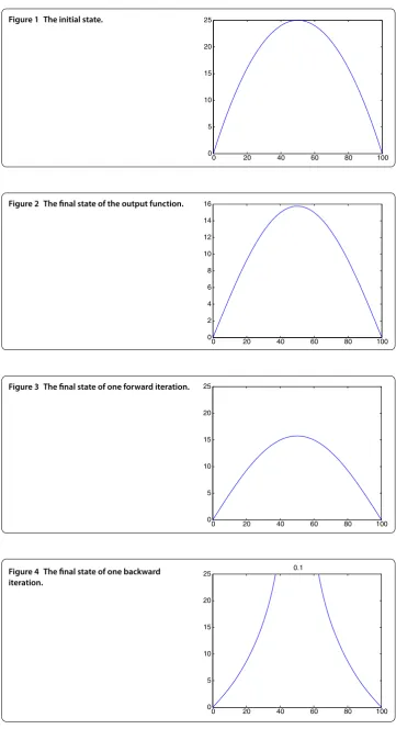
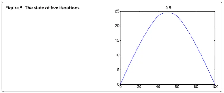
In order to show the efficiency of the iterative algorithm, we consider the particular case where= [, ],O= [, ], t= τ
T,T= ,a= ,h= ., and the initial data to
be recover isz=x( –x)/. We use a Crank-Nicolson scheme and quasi-reversible method of regularization inverse inversion to simulate the observer systems (.) and (.) from one iteration to multiple iterations in time combined with a finite difference space discretization. Figure shows the initial state, Figure shows the final evolution of the output function. After one forward and backward iteration, we can obtain Figure and Figure , obviously the result is not accurate enough, and after five iterations we obtain Figure . Figure shows that the recursive algorithm reconstructs the initial state as far as possible. The algorithm take the simplest system and still needs to be improved.
7 Conclusion
The above iterative algorithm by using the forward and backward observers may esti-mate the initial state of the inverse problems of the nonlinear system under certain con-ditions. The numerical convergence accuracy analysis based on observers in the semi-discretization and the full-semi-discretization can also be obtained. The convergence analysis ofz,handz,h, ttowardsz,hhas been showed for the nonlinear system if the truncation
parametersNhandNh, tare optimal. The estimate error we have got provides the
Figure 1 The initial state.
Figure 2 The final state of the output function.
Figure 3 The final state of one forward iteration.
Figure 5 The state of five iterations.
and demonstrates it in detail. We need to work on more applications of the algorithm and on the accuracy.
Competing interests
The authors declare that they have no competing interests.
Authors’ contributions
All authors contributed equally to the writing of this paper. All authors read and approved the final manuscript.
Acknowledgements
This work was supported by the National Natural Science Foundation of China. Grant No. 51205286.
Received: 30 September 2013 Accepted: 26 February 2014 Published:12 Mar 2014
References
1. Ramdani, K, Tucsnak, M, Weiss, G: Recovering the initial state of an infinite-dimensional system using observers. Automatica46(10), 1616-1625 (2010)
2. Auroux, D, Blum, J: A nudging-based data assimilation method: the Back and Forth Nudging (BFN) algorithm. Nonlinear Process. Geophys.15, 305-319 (2008)
3. Auroux, D, Blum, J: Back and forth nudging algorithm for data assimilation problems. C. R. Math. Acad. Sci. Paris340, 873-878 (2005)
4. Hoke, J, Anthes, A: The initialization of numerical models by a dynamic initialization technique. Mon. Weather Rev. 104, 1551-1556 (1976)
5. Liu, K: Locally distributed control and damping for the conservative system. SIAM J. Control Optim.35(5), 1574-1590 (1997)
6. Tucanak, M, Weiss, G: Observation and Control for Operator Semigroups. Birkhäuser Advanced Texts. Birkhäuser, Basel (2009)
7. Byungik, K: Multiple valued iterative dynamics models of nonlinear discrete-time control dynamical systems with disturbance. J. Korean Math. Soc.50, 17-39 (2013)
8. Curtain, RF, Zwart, H: An Introduction to Infinite-Dimensional Linear Systems Theory. Texts in Applied Mathematics, vol. 21. Springer, New York (1995)
9. Ramdani, K, Takahashi, T, Tenenbaum, G, Tucsnak, M: A spectral approach for the exact observability of infinite-dimensional systems with skew-adjoint generator. J. Funct. Anal.226, 193-229 (2005)
10.1186/1687-1847-2014-82
Cite this article as:Xie and Chang:Reconstructing the initial state for the nonlinear system and analyzing its