Volume 2010, Article ID 182627,13pages doi:10.1155/2010/182627
Research Article
A Multimedia Application: Spatial Perceptual Entropy of
Multichannel Audio Signals
Shuixian Chen,
1Ruimin Hu,
1, 2and Naixue Xiong
11Computer School, Wuhan University, Wuhan 430072, China
2National Engineering Research Center for Multimedia Software, Wuhan University, Wuhan 430072, China
Correspondence should be addressed to Naixue Xiong,[email protected]
Received 17 November 2009; Accepted 11 February 2010
Academic Editor: Liang Zhou
Copyright © 2010 Shuixian Chen et al. This is an open access article distributed under the Creative Commons Attribution License, which permits unrestricted use, distribution, and reproduction in any medium, provided the original work is properly cited.
Usually multimedia data have to be compressed before transmitting, and higher compression rate, or equivalently lower bitrate, relieves the load of communication channels but impacts negatively the quality. We investigate the bitrate lower bound for perceptually lossless compression of a major type of multimedia—multichannel audio signals. This bound equals to the perceptible information rate of the signals. Traditionally, Perceptual Entropy (PE), based primarily on monaural hearing measures the perceptual information rate of individual channels. But PE cannot measure the spatial information captured by binaural hearing, thus is not suitable for estimating Spatial Audio Coding (SAC) bitrate bound. To measure this spatial information, we build a Binaural Cue Physiological Perception Model (BCPPM) on the ground of binaural hearing, which represents spatial information in the physical and physiological layers. This model enables computing Spatial Perceptual Entropy (SPE), the lower bitrate bound for SAC. For real-world stereo audio signals of various types, our experiments indicate that SPE reliably estimates their spatial information rate. Therefore, “SPE plus PE” gives lower bitrate bounds for communicating multichannel audio signals with transparent quality.
1. Introduction
A central goal in multimedia communications is to deliver quality contents with the lowest possible bitrate. By quality, we mean the perceived fidelity of the received contents against the original contents. And the lowest possible bitrate depends on two disparate concepts: entropy and perception.
Entropy measures the quantity of information [1]. But not
all information is perceptible.
To pursue this goal, we want to know how many
bits are sufficient to convey quality multimedia contents.
Lossless compression always ensures the highest possible quality, in which the objective redundancy in the multimedia contents is the only source of compression, and there is a limit, the Shannon entropy, the lowest possible bitrate with perfect decompression. Nevertheless, this limit is very hard if not impossible to compute due to the diversity and complexity of probability models of multimedia contents.
By Huffman coding, run-length coding, arithmetic coding,
and other entropy coding techniques, the state-of-the-art lossless audio coders today typically achieve a compression
rate of 1/3-2/3 or 230–460 kbps per channel for CD music [2].
Lossless compression generally conveys higher than nec-essary quality in multimedia communications. Multimedia contents abound subjective irrelevancy—objective informa-tion we cannot sense. Perceptually lossless compression
suffices. For audio signals, this means lossless to the extent
that the distortion after decompression is imperceptible to normal human ears (usually called transparent coding), the bitrate can be much lower than the true lossless coding.
Perceptual audio coding [3] by removing the irrelevancy
greatly reduces communication bandwidth or storage space. Psychoacoustics provides a quantitative theory on this
irrelevancy [4–7]: the limits of auditory perception, such
as the audible frequency range (20–20000 Hz), the Absolute
Threshold of Hearing (ATH), and the masking effect [8]. In
state-of-the-art perceptual audio coders, such as MPEG-2/4
Advanced Audio Coding (AAC [9,10]), 64 kbps is enough
for transparent coding [11]. The Shannon entropy cannot
In 1988, Johnston proposed Perceptual Entropy (PE [12,
13]) for audio coding based on psychoacoustics. PE gives the
lower bitrate bound for perceptual audio coding:
PE= 1
where PE is measured in bits per sample,N the length of
block transform (usually DFT), nint() integer rounding, bi
the index of starting bin of subbandi,ωkthekth transform
coefficient, nithe undetectable distortion upper bound of
band,iandkithe number of bins in subbandi.Table 1lists
PE for various mono audio signals. The last column gives nears transparent bitrates of current coders, slightly lower than the upper bound of PE.
We can see that ifni in (1) assumes conservative values
(smaller), PE will be larger. On the other hand, Adaptive
Multirate (AMR [14]) and Adaptive Multirate Wide Band
(AMR-WB [15]) use a priori knowledge of human voicing,
also reducing bitrate. Apart from these two points, PE reliably predicts the lowest bitrate required for transparent audio coding. Since formulated, PE has found widespread use in audio coding and has become a fundamental theory in this field. Main stream perceptual audio coders, such as MP3
[16] and AAC, all employ PE as an important psychoacoustic
parameter, leading to various practical methods not just theory.
Nevertheless, PE has significant limitation to measure perceptual information. This limitation primarily comes from the underlying monaural hearing model. Human has two ears to receive sound waves in a 3-dimensional space: not only is the time and frequency information perceived— needing just individual ears—but also spatial information or localization information—needing both ears for spatial sampling. Due to the unawareness of binaural hearing, PE of multichannel audio signals is simplified to the supposition of PE of individual channels, which is significantly larger than real quantity of information received because multichannel audio signals usually correlate. The purpose of this paper is to measure the perceptual information of binaural hearing.
We first analyze the localization principle of binaural hearing and give a spatial hearing model on the physical and physiological layers. Then we propose a Binaural Cue Physiological Perception Model (BCPPM) based on binaural hearing. Finally using binaural frequency-domain perception property, we give a formula to compute the quantity of spatial information and numerical results of spatial information estimation of real-world stereo audio signals.
With the left and right ears, human being is able to detect spatial information: sound source localization and sound source spaciousness. The former comprises of the range, azimuth, and elevation, in other words, the 3-dimensional spherical coordinate. The later can be measured by angle span of auditory images.
Other
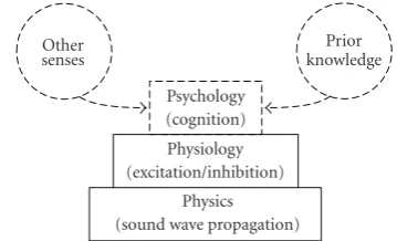
Figure1: 3 Layers of auditory sound source localization.
Human spatial hearing is a complex procedure of physics,
physiology, and psychology (Figure 1). Psychology stays
on the top of this procedure. On this layer, hearing is transformed to cognition, substantially influenced by subject psychological state, other senses, especially visual perception, and knowledge, implying that the same sound does not
necessarily produce the same hearing perception. InSpatial
Hearing, Blauert gives examples that different subjects in the same sound environment have diverse description of the
environment [17]. In 1998, Hofman et al. reported inNature
that subjects with modified pinnae shape lost the elevation detection ability at the beginning but gradually regained
that full ability [18]. This phenomenon demonstrates that
the subjects were able to learn the correspondence between frequency response characteristics with the modified pinnae
and sound from different elevations and used the knowledge
to guide elevation detection. Due to the above reasons, spatial hearing on the psychological layer is too complicated to be exploited in audio compression systems, which cannot assume any specific states, senses, and knowledge of listeners. On the physical layer, sound waves propagate from
sources along different paths to the ears and then in the
ear canals and finally to the cochlea, absorbed and reflected by walls, floors, torso, head, and other objects on the way. Those sound waves carry objective localization information. On the physiological layer, sound waves are transformed to neural cell excitation and inhibition by the auditory
system. There are different types of auditory neural cell
responding to different types of sound stimulus, such as
intensity, frequency, and delay. Thus physical quantities become physiological data.
In audio compression, irrelevancy removing is mainly on the physical and physiological layers. In the following, we discuss the representation of binaural cues on the two layers—BCPPM.
1.1. Spatial Information on the Physical Layer. As early as 1907, Rayleigh studied the physics of spatial hearing
[19]: Interaural Time Difference (ITD) and Interaural Level
Difference (ILD). Also Rayleigh has two seminal discoveries:
the famous duplex theory, that is, below 1.5 kHz, ITD is the primary localization cue and above 1.5 kHz ILD instead,
the head-shadow effect, that is, the blocking and reflection
Table1: PE and bitrate of various mono audio signals [13].
Sampling Rate (kHz) Band Width (kHz) PE (bits/sample) Bitrate (kbps) Near Transparent Coding Bitrate (kbps)
8 0.2–3.2 0.5–2.1 4–16.8 12.2 (AMR [14])
16 0–7 0.5–2.1 8–33.2 23.85 (AMR-WB [15])
32 0–15 0.35–2.1 9.6–67.2 64 (AAC [9])
Plane wave
Figure2: The rigid ball model of human head used by Rayleigh.
difference. Both discoveries are derived based on the rigid
ball modeling of head (Figure 2).
2. Physiological Perception Modeling of
Binaural Hearing
Although a real head is far from being the rigid ball, the above results are basically correct. In 2002, Macpherson and Middlebrooks demonstrated that the duplex theory is suitable for a variety of audio signals: pure tones, wide band
signals, high pass signals, as well as low pass signals [20].
Exception is high frequency signals with envelope delay [17].
ITD and ILD are not all the localization cues. On the medial plane (which cuts perpendicularly through the middle of the line connecting the left and right ears), all
sound sources have ITD=0 ms and ILD = 0 dB. But when
they have different elevations, our auditory system can detect
the difference by elevation-related spectral characteristics
[21–24]. Due to the asymmetric structure of pinnae [25],
the interference of sound waves is both wavelength related
and elevation related (Figure 3). For example, the frequency
of the lowest spectral amplitude (interference annihilation)
is a function of the elevation [26]. This is the root of our
elevation detection ability. This spectral cue does not depend on binaural hearing, so it is also called monaural cue.
Unlike ILD and ITD, the spectral cue needs prior knowledge to provide elevation information. In principle, sounds may have arbitrary spectra. A listener is not able to detect the elevation angle based solely on the spectra: any characteristics may come from sound sources themselves and
may come from the filtering effect of pinnae. The listener
cannot tell.
Blauert reported a very interesting auditory phenomenon of narrow-band sound sources on the medial plane: the elevation angles given by subjects are independent of the
real elevation angles but depended on the signal frequencies
[17]. For wide-band signals of familiar types, it is easy for
our auditory system to compare the pinnae filtered spectra (some frequency amplified and some decayed) to the spectra
in memory, and based on the difference, reliable elevation
angle estimation can be given (Figure 3). But for
narrow-band signals, pinnae filtered spectra do not have detectable
shape difference, just level difference. Thus the elevation
angle detection will be very unreliable. In fact, the elevation angles given by the subjects are the angles at which the narrow-band signals have the maximum gain due to the pinnae filtering. For example, the peak gain frequency when the sounds come from the front is 3 kHz for most people
[21]. So wherever a sound of 3 kHz came from, most subjects
pointed at the front.
From the perspective of signal processing, sound wave propagation is roughly a Linear Time Invariant (LTI) system. To describe this LTI system in binaural hearing, we have
Head-Related Transfer Function (HRTF [27–29]) or
equiv-alently Head-Related Impulse Response (HRIR). In open space, HRTF/HRIR is the function of source location, that is, range, azimuth, and elevation.
Figure 4 shows the HRTFs in binaural hearing. Signal
S(jω) goes from the source though the left and right paths
to the left and right ears, respectively. Denote byHlθ(jω) the
spectra, localization cannot be determined solely bySθ
l(jω)
orSθ r(jω).
Suppose that there are no strict zeros in the signal and
the HRTFs. To exclude the effect ofS(jω), we define Binaural
Difference Transfer Function (BDTF):
Hθ
which is independent ofS(jω) and located related. BDTF
contains the same spatial information asSθl(jω) andSθr(jω).
In fact, we can find ILD and ITD from it:
ILD=20log10 Hθ
Obviously, ILD and ITD are not only source location dependent, but also frequency dependent.
Up
(a)
Front
(b)
−20 0 10 20
(dB)
0.1 1 10
Frequency (kHz) (c)
−20 0 10 20
(dB)
0.1 1 10
Frequency (kHz) (d)
Figure3: Elevation angle detection (Modified fromhttp://interface.cipic.ucdavis.edu/CIL tutorial/3D psych/elev.htm).
Lab collected HRTFs on 710 locations in the 3-dimensional
space using the KEMAR head [30]. In 2001, CIPIC of
U.C. Davis examined HRTFs of 45 subjects and 2 KEMAR
heads [31]. Individual difference of HRTFs is revealed in
HRTFs obtained by the experiments. Nevertheless, there are
common characteristics that are sufficient to derive
subject-independent spatial information.
2.1. Spatial Information on the Physiological Layer. In human auditory system, ITD and ILD of external sound sources stimulate or inhabit specific neural cells in the full audible frequency range. This process comprises of two steps:
Frequency-to-Place Transform (FPT) [32,33] and Binaural
Processing (BP).
In 1960, B`ek`esy reported that sounds of different
fre-quencies generate surface waves on the basilar membrane
in cochlea with peak amplitudes at different places, which
are determined by the frequencies [34]. In other words, a
specific frequency is mapped to a specific place on the basilar membrane, or FPT, and this specific frequency for a given
place is called Characteristic Frequency (CF [35]). Hair cells
on that place then transform the mechanical swing into electric signals of auditory nerves.
Hθ r(jω)
Hθ l(jω)
Hlθ(jω)
Hθ r(jω)
S(jω)
Hθ r(jω)S(jω)
Hlθ(jω)S(jω)
θ
Figure4: Binaural hearing transfer functions.
Output 1 Output 2 Outputn−1 Outputn
× × × ×
ΔT ΔT ΔT
ΔT ΔT ΔT Right ear in
Left ear in
· · ·
Figure5: Jeffress model: delay line network.
this process: Excitation-Excitation (EE [36]) and
Excitation-Inhibition (EI [37]). The former proposed that there are
auditory nerve cells of EE-type located between the inferior colliculus and the medial superior olive, and specific EE-type cells there have maximum excitation for signals with specific ITD and ILD; the latter proposed that there are auditory nerve cells of EI-type located between the inferior colliculus and the lateral superior olive, and specific EI-type cells there have maximum inhibition for signals with specific ITD and ILD. The common ground of the two theories is that specific nerve cells are only sensitive to specific ITD and ILD, which are called characteristic ITD and characteristic ILD. In some literatures, characteristic ITD is also called Best Delay
(BD [38]) or Characteristic Delay (CD [39]). Both the
EE-type and EI-EE-type have supports from physiological research, but the latter explains better the various binaural hearing
phenomena [40].
In 1948, Jeffress gave a physiological model for ITD
perception [41, 42]—delay line model—the foundational
contribution, having lasting impact in the field (Figure 5).
Neural signals in the form of spike train from the left and right auditory pathways meet at some coincidence counter after traveling along the left and right delay lines and trigger the counter, which is in fact a physiological cross-correlation calculator. The specific counter having the largest counts is
the counter to which the delay difference along the left and
right delay lines exactly compensates the ITD. For example,
sounds from the medial plane (ITD=0) generate the largest
counts in the middle counter of the Jeffress network. The
coincidence counters can be classified as EE-type auditory nerve cells.
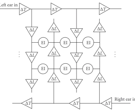
In 2001, Breebaart et al. extended the Jeffress model by
incorporating attenuators [43–45] (Figure 6). An important
difference to the Jeffress model is the use of EI-type elements
instead of the EE-type elements in the Breebaart model. Due to the attenuators, ILD can be extracted by the extended model.
In the Breebaart model, only if the internal delay and attenuation are exactly compensated by the external ITD and ILD, the corresponding EI-type elements will have the largest inhibition. Thus, knowing the position of the EI-type element with the largest inhibition, the auditory system finds the ITD and ILD of the external audio signals.
The Breebaart model also implies the calculation of Interaural Coherence (IC), which manifests as the trough
ΔT ΔT ΔT
ΔL ΔL ΔL ΔL
EI EI EI
ΔL ΔL ΔL ΔL
EI EI EI
ΔL ΔL ΔL ΔL
ΔT ΔT ΔT Right ear in
Left ear in
. . . .
. .
Figure6: Breebaart model: delay-attenuation network.
of the excitation surface, in accordance with the EI-type assumption. Nevertheless, there is no direct physiological quantity related to IC in this model.
In 2004, Faller and Merimma reported that IC relates to perceiving sound image width and stability, as well as sound
field ambience [46,47]. On the other hand, by the precedence
effect [48,49] of spatial hearing—sound source localization
depending primarily on the direct sounds to the ears and essentially irrespective to reflection and reverberation— which contributes to lowering IC, Faller proposed that our auditory system use ITD and ILD to localize sound sources only if IC approaches 1. Since direct sounds to the ears have
near 1 cross-correlation, this explains the precedence effect.
2.2. Binaural Cue Physiological Perception Model (BCPPM). From the viewpoint of the information theory, the channel from the physical layer to the physiological layer is lossy, and less spatial information survives during the course (Figure 7).
Since the wavelength (0.012–17 m) of sound in the audible range (20–20000 Hz) is much longer than light, and comparable to normal objects in our surrounding—
leading to significant interference and diffraction—spatial
information from hearing is limited initially. This limited information is first compromised by noises and other
interferences from other sound sources, as indicated byΔp1
in Figure 7. Then during transformation from mechanical swing to electric impulses, part of the information is lost again due to the limited frequency range and dynamic range, the limited frequency and temporal resolution, and physiological noises of our auditory system, as is indicated byΔp2inFigure 7.
The loss of spatial information manifests as offset and
Sound
Figure7: Spatial information loss.
auditory filtering cannot separate them. And the perceived
ITD and ILD are determined by the combined effects of
BDTFs of those sources, typically leading to biased and
vaguer location perception (Figure 8). A large sound source
has similar localization effects. In the Breebaart model, the
resolution of ITD and ILD is limited by the fineness of the delay elements and attenuation elements: no ITD smaller
than the delay offered by one delay element can be detected
and no ILD smaller than the attenuation offered by one
attenuation element can be detected. This is in analogy to the ATH in monaural hearing. The limited ITD and ILD resolution turns out to limited localization resolution.
In Section 1.1, we see that the physical data of sound source localization in binaural hearing are in form of
ITD and ILD. In Section 2.1, we see that ITD and ILD
are transformed to maximum inhibition of specific EI-type auditory nerve cells in the Breebaart model, and the physiological data are in the form of coordinates of the delay-attenuation network.
When there are multiple sound sources, background
noises, reflection, diffraction, and reverberation, IC becomes
another type of physical data conveying the overall sound field information.
Since spatial hearing on the physiological layer is too complex and uncertainty to be incorporated in computa-tional model for common listeners, we restrict the calcula-tion of perceptible spatial informacalcula-tion to that directly related to ITD, ILD, and IC and physiological data corresponding to the three cues. In fact, spatial coding systems use the cues to represent spatial information.
We first review the psychoacoustic foundation of PE, mainly the nonlinear frequency resolution (Critical Band,
CB [50, 51]) of our hearing system, spreading functions
in the frequency domain for noises and tones and tonality estimation.
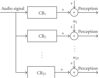
To calculate PE, Johnston used a Monaural Hearing
Model (MHM, Figure 9). In this model, a 25-subband
filterbank filters incoming audio signals. Each subband has a
bandwidth of CB at the corresponding frequency (CB1-CB25
in Figure 9), increasing from low to high frequency. Each subband also acts as a lossy subchannel, and the loss of audio information is due to the intrinsic noises of hearing system
(ATH) and interchannel interference (masking effect). ATH
is signal dependent, usually as a table or a fitting function of experimental data. Masking is signal dependent, usually obtained by convoluting the tonality-dependent spreading functions with the signal spectra. Combining both, we have effective channel noises (n1-n12inFigure 9).
Figure8: Two types of spatial information loss.
Audio signal Perception
Figure9: Monaural Hearing Model (MHM) used to calculate PE.
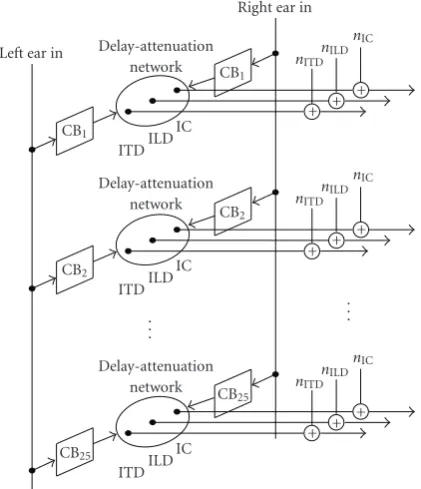
There is no place for localization in the MHM. The critical limit of the model is the lack of binaural processing— only spectral-temporal information but not spatial informa-tion. The Breebaart delay-attenuation network just models the binaural processing. So we borrow the idea of lossy multichannel in MHM and combine MHM with the Bree-baart model—Binaural Cue Physiological Processing Model
(BCPPM,Figure 10).
The BCPPM consists of 3 modules.
Frequency-to-Place Transform in Cochlea. This process sep-arates sounds into a bank of subband signals, essentially the subband filtering in MHM. The subband filter can be implemented by DFT with spectral lines grouped to subbands according to CB or by the Cochlear Filter Bank
(CFB [52]) proposed by Baumgarte in 2002.
Delay-Attenuation Network. This is the same as that in Figure 6. After the Time-to-Place Transform, external audio signals change into spike trains of auditory nerve signals, which arrive at the corresponding delay-attenuation net-works. Then the networks output ITD, ILD, and IC for each critical band. From the location of the maximum inhibition (lowest excitation, the trough of the neural excitation surface inFigure 11), we can derive ITD and ILD. From the gradient of the trough, we can derive IC: faster descending or larger
gradient implies larger IC (≤ 1); slower descending or
CB25
CB2
CB1
Left ear in Delay-attenuation network
Figure10: Binaural Cue Physiological Perception Model (BCPPM).
Effective Channel Noises. The effective channel noise for
ITD, ILD, and IC (nITD, nILD, and nIC in Figure 10) is a
simplified method to model the limited precision, intrinsic noises, and intersource interference in our hearing system. Part of the noise comes directly from grains of delay and
attenuation (ΔT andΔLinFigure 6). For example, ifΔT =
10μs,nILD ≥ 10μs. Generally,ΔT andΔLare functions of
frequency. A related concept is Just Noticeable Difference
(JND) in psychoacoustics, indicating the overall sensitivity of our auditory system. On the other hand, ITD, ILD, and IC are not independent, there are interactions among
them. The effective channel noise should also incorporate the
interactions.
3. Computing Spatial Perceptual Entropy (SPE)
Based on BCPPM
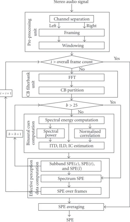
In this section, we will define SPE using the BCPPM and then discuss in detail the computational implementation of BCPPM, including 3 core components: the CB filterbank, binaural cues computation, and perceptible information
computation (Figure 12).
3.1. SPE Definition . From the information theory view-point, we see BCPPM as a double-in-multiple-out system (Figure 10). The double-in is the left ear entrance sound and the right ear entrance sound. The multiple-out consists of 75
effective ITDs, ILDs, and ICs (25 CBs, each with a tuple of
ITD, ILD, and IC).
Like in computing PE, we view each path that leads to an output as a lossy subchannel. Then there are 75 such subchannels. Unlike PE, what a subchannel conveys is not
0
Figure11: An example of auditory nerve excitaton surface with
ITD=0 ms and ILD=0 dB, adapted from [42].
a subband spectrum but one of ITD, ILD, and IC of the subband corresponding to the sub-channel.
In each sub-channel, there are intrinsic channel noises (resolution of spatial hearing), and among sub-channels, there are interchannel interferences (interaction of binaural
cues). Then there is an effective noise for each sub-channel.
Under this setting, each sub-channel will have a channel
capacity. We denote SPE(c), SPE(t), and SPE(l) for the
capacity of IC, ITD, and ILD sub-channels respectively. Then SPE is defined as the overall capacity of these sub-channels, or the sum of capacities of all the sub-channels:
SPE=
all subbands
SPE(c) + SPE(t) + SPE(l). (4)
To derive SPE(c), SPE(t), and SPE(l), we need probability
models for IC, ITD, and ILD. Although the binaural cues are
continuous, the effective noise quantizes them into discrete
values. Let [L·P], [T·P], and [C·P] denote the discrete ILD, ITD, and IC source probability spaces:
[L·P] :
probabilities. Then we have
Table2: Critical Bands for 2048-point DFT, sampling frequency 48 kHz [40].
CB Index Frequency Range (Hz) Spectral Index CB Index Frequency Range (Hz) CB Index
1 0∼100 0∼3 14 2000∼2320 85∼98
2 100∼200 4∼8 15 2320∼2700 99∼114
3 200∼300 9∼12 16 2700∼3150 115∼133
4 300∼400 13∼16 17 3150∼3700 134∼157
5 400∼510 17∼21 18 3700∼4400 158∼187
6 510∼630 22∼26 19 4400∼5300 188∼225
7 630∼770 27∼32 20 5300∼6400 226∼272
8 770∼920 33∼38 21 6400∼7700 273∼328
9 920∼1080 39∼45 22 7700∼9500 329∼404
10 1080∼1270 46∼53 23 9500∼12000 405∼511
11 1270∼1480 54∼62 24 12000∼15000 512∼639
12 1480∼1720 63∼72 25 15000∼24000 640∼1023
13 1720∼2000 73∼84 — — —
For some probability distributions, say uniform distribution, (5), (6), and (7) can be readily calculated.
3.2. CB Filterbank. We use the same method as that in PE to implement the CB filterbank. Audio signals are first transformed to the frequency domain by DFT of 2048 points with 50% overlap between adjacent transform blocks. Then a
DFT spectrum is partitioned into 25 CBs according toTable 2
[41]. Then basic processing unit is the subspectra of each CB.
3.3. Binaural Cues Computation. ILD is the ratio of left ear entrance signal intensity to right ear entrance signal intensity. Since DFT preserves signal energy, we can use DFT
subspectra energy ratio to compute ILD on each CB [53]:
ILD(b)=20log10
Xr(k)thekth spectral lines from left and right ear entrance
signals.
Time shift corresponds to linear phase shift in the frequency domain. Therefore, we can use group delay (slope of phase-frequency curve) of subband signal to derive ITD on each subband:
represents the phase of a complex number. A more reliable
but also more complex method is to use least square fitting to find the group delays and then ITD:
ITD(b)=wb
Due to the property that time-domain normalized correlation is equivalent to the real part of correlation in the frequency domain, IC of each CB can be derived as the following:
3.4. Effective Spatial Perception Data . The resolutions or
quantization steps of the binaural cues (Figure 12) can be
determined by JND experiments. Denote byΔτ,Δλ, andΔη
the resolutions of ITD, ILD, and IC, respectively. Generally, they are signal dependent and frequency dependent. For
simplicity, we use constant values [44,54]: Δτ = 0.02 ms,
Δλ=1 dB, andΔη=0.1.
IC has different impacts on ITD and ILD perception. In
2001, Hartmann Constan reported that the difference of JND
of ILD for correlated noises and uncorrelated noises is only
0.5 dB [55]. This can be explained by the fact that signal
power is independent phase, which influences correlation, and lower IC is partly the result of increasing phase noise.
This is illustrated in Figure 13: when IC decreases, the
gradient along the ILD axis keeps almost unchanged, but the gradient along the ITD significantly decreases.
Resolution of spatial hearing
Figure12: SPE calculation.
−10
Figure13: The different effects of IC on ITD and ILD perception.
approaches 1, the activity surface will have a very sharp decreasing toward the point with the lowest auditory nerve activity. In this case, the uncertainty of ITD is very small and is determined precisely. When IC decreases to 0, the surface becomes flatter, leading to larger uncertainty or
lower precision of ITD. In the extreme case, when IC = 0,
the gradient along the IC axis will be constantly 0, there is no well defined trough point and ITD is completely indeterminable.
By the above analysis, we ignore the effect of IC on
ILD and only consider the effect of IC on ITD for SPE
computation. Lower IC leads to lower resolution of ITD. This
is equivalent to higher JND of ITD. Then the effective JND
on subbandb, denoted asΔτ(b), can be formulated as the
following:
Δτ(b)=Δτ(b)
IC(b). (13)
From (13) we see that when IC(b)=1,Δτ(b) assumes
the minimumΔτ(b) and the auditory system has the highest
resolution for ITD; when 0<IC(b)<1,Δτ(b)<Δτ(b)<
∞, the resolution of ITD is lower but there is still spatial
information from ITD; when IC(b) = 1,Δτ(b) = ∞, the
resolution of ITD is 0 and there is no spatial information in ITD.
Then we have the following effective perception data
qILD(b),qITD(b), andqIC(b) of ILD, ITD, and IC, respectively
where· represents the round down function.
Suppose thatqILD(b),qITD(b), andqIC(b) are uniformly
whereNis the number of spectral lines in one transform, or
1024 in this case; ILD(b), ITD(b), and IC(b) can be found
from (9), (10), and (11), respectively; Δλ(b), Δτ(b), and
Δη(b) are the JNDs of ILD, ITD, and IC on CBb,respectively,
obtained from subjective listening experiments; andαis the
amplitude compression factor, assuming 0.6 [5].
4. Experiments
SPE
ITD, ILD, IC estimation Spectral
i >overall frame count Windowing
Figure14: Flowchart of SPE Computation.
Figure 14 gives the computational procedure of SPE: stereo audio signals are windowed and block transformed to the frequency domain using 2048-point DFT; then on the 25 CBs, binaural cues are derived before transformed into
effective spatial perception data, the entropy of which is SPE.
In the following experiments,Δτ(b),Δλ(b), andΔλ(b) assume constant and conservative values, and their frequency dependency is also ignored. The overall SPE is the sum of
entropy of effective IC, ILD, and ITD perception data, shown
in (4).
4.1. Perceptual Spatial Information of Stereo Sequences. In this experiment, we compute perceptual spatial information by
SPE for 4 classes of stereo sequences (Figure 15): each class
consists of 12 sequences, sampled at 44.1 kHz; each data point is average of SPE over one sequence, measured by kbps. FromFigure 15we find that speech sequences generally have the lowest spatial information rate, mean 2.75 kbps, this is in accordance with the recording practice that voices usu-ally stay in direct front of the sound field; single instrument
4.11 Single instrument, mean=3.49
Figure 15: Perceptual spatial information of stereo sequences sampled at 44.1 kHz.
sequences and simple mixture sequences have similar spatial information rate, mean 3.49 kbps and 3.66 kbps, respectively; complex mixture sequences generally have the highest spatial information rate, mean 6.90 kbps, this can be explained by multiple sound sources at diverse sound field locations in this type of sequences.
In Parametric Stereo (PS [56]) coding, it is reported
that 7.7 kbps of spatial parameter bitrate is sufficient for
transparent spatial audio quality, agreeing very well with our SPE computation.
4.2. Temporal Variation of Spatial Information Rate in a Single Senescence. In this experiment, we choose two sequences es02 of German male speech and sc03 of contemporary pop music from MPEG and compute their SPE frame by frame (Figure 16).
The test data show that for es02 with stable voice from the front, SPE stays at 1-2 kbps; for sc03 with multiple instruments and strong spatial impression, SPE stays at about 7 kbps. But within either sequence, the SPE changes little.
4.3. Overall Perceptual Information in Stereo Sequences. Using PE to evaluate the perceptual information, only intrachannel redundancy and irrelevancy are exploited; the overall PE is simply the sum of PE of the left and right channels. Using SPE based on BCPPM, interchannel redundancy and irrelevancy are also exploited; the overall perceptual information is about one normal audio channel plus some spatial parameters, which has significantly lower bitrate.
For the above reason, PE gives much higher bitrate
bound than SPE (Figure 17). PE is compatible with the
traditional perceptual coding schemes, such as MP3 and AAC, in which channels are basically processed individually (except the mid/side stereo and the intensity stereo). So PE gives meaningful bitrate bound for them. But in Spatial
Audio Coding (SAC [52, 54, 57–59]), multichannel audio
(a) (b)
0 1 2 3 4 5 6 7
SP
E
(kbps)
0 1 2 3 4 5 6
Time (s) (c)
0 1 2 3 4 5 6 7
SP
E
(kbps)
0 1 2 3 4 5 6 7 8 9 10
Time (s) (d)
Figure16: SPE of es02 (speech) and sc03(pop). (a): waveform of es02; (b): SPE curve of es02; (c): waveform of sc03; (d): SPE curve of sc03.
0 1 2 3 4 5 6 7
Ov
er
al
l
infor
mat
ion
ra
te
(bits/sample)
Simple mixture
Complex mixture
Speech Single instrument PE + PE
PE + SPE 4.2
2 6
3.3 2.3
1.5 2.8
1.6
Figure17: Perceptual Information of stereo sequences sampled at 44.1 kHz, evaluated using PE and SPE.
parameters. SPE is necessary in this case and generally gives
much lower bitrate bound (∼1/2). This agrees to the sharp
bitrate reduction of SAC.
5. Conclusion
We have developed the Binaural Cues Physiological Per-ceptual Model (BCPPM) to measure the perceptible information, or Spatial Perceptual Entropy (SPE), in multi-channel audio signals and have given a lower bitrate bound
in multimedia communications for this type of contents. BCPPM models the physical and physiological processing of human spatial hearing into a parallel of lossy communication subchannels with inter-subchannel interference, and SPE is the overall channel capacity. Each of these subchannels carries ITD, ILD, or IC with addictive noises, resulted from intrinsic noises of binaural cues perception and interferences among the cues within the same CB. Experiments on
stereo signals of different types have confirmed that SPE
is compatible with the spatial parameter bitrate and spatial impression in SAC.
Nevertheless, SPE gives only the lower bitrate bound for transparent quality. We will extend SPE to give the bound for given subjective quality in the future. Then in mobile, internet, and other communications networks conveying multichannel audio signals, we can use the estimated bound to allocate bandwidth for a particular Quality of Service (QoS), transparent or degraded and thus save bandwidth or improve the overall QoS. On the other hand, current SAC may benefit from SPE—dynamically allocating bitrate to accommodate varying spatial contents—thus improving quality and reducing overall bitrate.
Acknowledgment
References
[1] C. E. Shannon, “A mathematical theory of communication,” Bell System Technical Journal, vol. 27, pp. 379–423, 623–656, 1948.
[2] “Lossless comparison,” http://wiki.hydrogenaudio.org/index
.php? title=Lossless comparison.
[3] T. Painter and A. Spanias, “Perceptual coding of digital audio,” Proceedings of the IEEE, vol. 88, no. 4, pp. 451–513, 2000.
[4] E. Zwicker and H. Fastl, Psychoacoustics Facts and Models,
Berlin, Germany, Springer, 1990.
[5] B. C. J. Moore,An Introduction to the Psychology of Hearing,
Elsevier Academic Press, London, UK, 5th edition, 2003. [6] E. Zwicker and U. T. Zwicker, “Audio engineering and
psychoacoustics. Matching signals to the final receiver, the
human auditory system,” Journal of the Audio Engineering
Society, vol. 39, no. 3, pp. 115–126, 1991.
[7] J. L. Hall, “Auditory psychophysics for coding applications,” in The Digital Signal Processing Handbook, V. Madisetti and D. Williams, Eds., pp. 39.1–39.25, CRC Press, Boca Raton, Fla, USA, 1998.
[8] B. C. J. Moore, “Masking in the human auditory system,” in Collected Papers on Digital Audio Bit-Rate Reduction, N. Gilchrist and C. Grewin, Eds., pp. 9–19, Audio Engineering Society, New York, NY, USA, 1996.
[9] ISO/IEC JTC1/SC29/WG11, “Information Technology— Generic Coding of Moving Pictures and Associated Audio Information—Part 7: Advanced Audio Coding (AAC),” ISO/IEC 13818-7, 2005.
[10] ISO/IEC JTC1/SC29/WG11, “Information Technology— Generic Coding of Moving Pictures and Associated Audio Information—Part 3: Audio, Subpart 4: General Audio Coding,” ISO/IEC 14496-3, 2005.
[11] M. Bosi and R. E. Goldberg, Introduction to Digital Audio
Coding and Standards, Kluwer Academic Publishers, Boston, Mass, USA, 2003.
[12] J. D. Johnston, “Transform coding of audio signals using
perceptual noise criteria,” IEEE Journal on Selected Areas in
Communications, vol. 6, no. 2, pp. 314–323, 1988.
[13] J. D. Johnston, “Estimation of perceptual entropy using noise
masking criteria,” inProceedings of IEEE International
Confer-ence on Acoustics, Speech and Signal Processing (ICASSP ’88), pp. 2524–2527, May 1988.
[14] 3GPP, “Mandatory speech CODEC speech processing func-tions; AMR speech Codec; General description,” 3GPP
TS 26.071, 2008, http://www.3gpp.org/ftp/Specs/html-info/
26071.htm.
[15] 3GPP, “Speech codec speech processing functions; Adaptive Multi-Rate—Wideband (AMR-WB) speech codec; General
description,” 3GPP TS 26.171, 2008,http://www.3gpp.org/ftp/
Specs/html-info/26171.htm.
[16] ISO/IEC and JTC1/SC29/WG11 MPEG, “Information tech-nology—coding of moving pictures and associated audio for digital storage media at up to about 1.5 Mbit/s—part 3: audio,” ISO/IEC 11172-3, 1992.
[17] J. Blauert,Spatial Hearing: The Psychophysics of Human Sound
Localization, MIT Press, Cambridge, Mass, USA, 1997. [18] P. M. Hofman, J. G. A. Van Riswick, and A. J. Van Opstal,
“Relearning sound localization with new ears,”Nature
Neu-roscience, vol. 1, no. 5, pp. 417–421, 1998.
[19] J. W. Strutt, “On our perception of sound direction,”
Philo-sophical Magazine, vol. 13, pp. 214–232, 1907.
[20] E. A. Macpherson and J. C. Middlebrooks, “Listener weight-ing of cues for lateral angle: the duplex theory of sound
localization revisited,” Journal of the Acoustical Society of
America, vol. 111, no. 5, pp. 2219–2236, 2002.
[21] J. Blauert, “Sound localization in the median plane,”Acustica,
vol. 22, no. 4, pp. 205–213, 1969-1970.
[22] J. Hebrank and D. Wright, “Spectral cues used in the
localization of sound sources on the median plane,”Journal of
the Acoustical Society of America, vol. 56, no. 6, pp. 1829–1834, 1974.
[23] R. A. Butler and K. Belendiuk, “Spectral cues utilized in the
localization of sound in the median sagittal plane,”Journal of
the Acoustical Society of America, vol. 61, no. 5, pp. 1264–1269, 1977.
[24] B. Rakerd, W. M. Hartmann, and T. L. McCaskey, “Identifi-cation and localization of sound sources in the median sagittal
plane,”Journal of the Acoustical Society of America, vol. 106, no.
5, pp. 2812–2820, 1999.
[25] A. D. Musicant and R. A. Butler, “The influence of
pinnae-based spectral cues on sound localization,” Journal of the
Acoustical Society of America, vol. 75, no. 4, pp. 1195–1200, 1984.
[26] F. Asano, Y. Suzuki, and T. Sone, “Role of spectral cues in
median plane localization,”Journal of the Acoustical Society of
America, vol. 88, no. 1, pp. 159–168, 1990.
[27] H. Møller, M. F. Sørensen, D. Hammershøi, and C. B. Jensen,
“Head-related transfer functions of human subjects,”Journal
of the Audio Engineering Society, vol. 43, no. 5, pp. 300–321, 1995.
[28] H. Møller, “Fundamentals of binaural technology,” Applied
Acoustics, vol. 36, no. 3-4, pp. 171–218, 1992.
[29] “Spatial hearing,” in Audio Signal Processing for
Next-Generation Multimedia Communication Systems, Y. Huang and J. Enesty, Eds., chapter 13, section 2, pp. 345–370, Kluwer Academic Publishers, Norwell, Mass, USA, 2004.
[30] W. G. Gardner and K. D. Martin, “HRTF measurements of a
KEMAR,”Journal of the Acoustical Society of America, vol. 97,
no. 6, pp. 3907–3908, 1995.
[31] V. R. Algazi, R. O. Duda, D. M. Thompson, and C. Avendano,
“The CIPIC HRTF database,” inProceedings of IEEE Workshop
on Applications of Signal Processing to Audio and
Electroacous-tics, pp. 99–102, New Paltz, NY, USA, October 2001.
[32] D. D. Greenwood, “A cochlear frequency-position function for
several species: 29 years later,”Journal of the Acoustical Society
of America, vol. 87, no. 6, pp. 2592–2605, 1990.
[33] D. D. Greenwood, “Critical bandwidth and the frequency
coordinates of the basilar membrane,” Journal of Acoustic
Society America, vol. 33, no. 10, pp. 1344–1356, 1961.
[34] G. von B`ek`esy,Experiments in Hearing, McGraw Hill, New
York, NY, USA, 1960.
[35] A. R. Møller,Hearing: Anatomy, Physiology, and Disorders of
the Auditory System, Academic Press, Burlington, Vt, USA, 2nd edition, 2006.
[36] J. E. Rose, N. B. Gross, C. D. Geisler, and J. E. Hind, “Some neural mechanisms in the inferior colliculus of the cat which
may be relevant to localization of a sound source,”Journal of
Neurophysiology, vol. 29, no. 2, pp. 288–314, 1966.
[37] T. J. Park, “IID sensitivity differs between two principal centers
in the interaural intensity difference pathway: the LSO and the
IC,”Journal of Neurophysiology, vol. 79, no. 5, pp. 2416–2431, 1998.
[38] P. X. Joris, B. Van de Sande, D. H. Louage, and M. van der
Heijden, “Binaural and cochlear disparities,”Proceedings of the
[39] R. M. Stern, DeL. Wang, and G. Brown, “Binaural sound
localization,” in Computational Auditory Scene Analysis, G.
Brown and DeL. Wang, Eds., Wiley/IEEE Press, New York, NY, USA, 2006.
[40] J. Breebaart, S. van de Par, and A. Kohlrausch, “The con-tribution of static and dynamically varying ITDs and IIDs
to binaural detection,” Journal of the Acoustical Society of
America, vol. 106, no. 2, pp. 979–992, 1999.
[41] L. A. Jeffress, “A place theory of sound localization,”Journal
of Comparative and Physiological Psychology, vol. 41, no. 1, pp. 35–39, 1948.
[42] P. X. Joris, P. H. Smith, and T. C. T. Yin, “Coincidence
detection in the auditory system: 50 years after Jeffress,”
Neuron, vol. 21, no. 6, pp. 1235–1238, 1998.
[43] J. Breebaart, S. van de Par, and A. Kohlrausch, “Binaural processing model based on contralateral inhibition. I. Model
structure,”Journal of the Acoustical Society of America, vol. 110,
no. 2, pp. 1074–1088, 2001.
[44] J. Breebaart, S. D. van de Par, and A. Kohlrausch, “Binaural processing model based on contralateral inhibition. II.
Depen-dence on spectral parameters,”Journal of the Acoustical Society
of America, vol. 110, no. 2, pp. 1089–1104, 2001.
[45] J. Breebaart, S. D. van de Par, and A. Kohlrausch, “Binau-ral processing model based on cont“Binau-ralate“Binau-ral inhibition. III.
Dependence on temporal parameters,”Journal of the Acoustical
Society of America, vol. 110, no. 2, pp. 1105–1117, 2001. [46] C. Faller and J. Merimaa, “Source localization in complex
listening situations: selection of binaural cues based on
interaural coherence,” Journal of the Acoustical Society of
America, vol. 116, no. 5, pp. 3075–3089, 2004.
[47] M. J. Goupell and W. M. Hartmann, “Interaural fluctua-tions and the detection of interaural incoherence: bandwidth
effects,”Journal of the Acoustical Society of America, vol. 119,
no. 6, pp. 3971–3986, 2006.
[48] P. M. Zurek, “The precedence effect,” inDirectional Hearing,
W. A. Yost and G. Gourevitch, Eds., pp. 85–105, Springer, New York, NY, USA, 1987.
[49] R. Y. Litovsky, B. Rakerd, T. C. T. Yin, and W. M. Hartmann, “Psychophysical and physiological evidence for a precedence
effect in the median sagittal plane,”Journal of Neurophysiology,
vol. 77, no. 4, pp. 2223–2226, 1997.
[50] H. Fletcher, “Auditory patterns,”Reviews of Modern Physics,
vol. 12, no. 1, pp. 47–65, 1940.
[51] B. Scharf, “Critical bands,” inFoundations of Modern Auditory
Theory, Academic Press, New York, NY, USA, 1970.
[52] C. Faller and F. Baumgarte, “Binaural cue coding—part II:
schemes and applications,”IEEE Transactions on Speech and
Audio Processing, vol. 11, no. 6, pp. 520–531, 2003.
[53] F. Baumgarte, “Improved audio coding using a psychoacoustic
model based on a cochlear filter bank,”IEEE Transactions on
Speech and Audio Processing, vol. 10, no. 7, pp. 495–503, 2002. [54] J. Breebaart, J. Herre, C. Faller, et al., “MPEG spatial audio
coding/MPEG surround: overview and current status,” inAES
119th Convention, New York, NY, USA, October 2005. [55] W. M. Hartmann and Z. A. Constan, “Interaural coherence
and the lateralization of noise by interaural level differences,”
Journal of the Acoustical Society of America, vol. 110, no. 5, p. 2680, 2001.
[56] J. Breebaart, S. van de Par, A. Kohlrausch, and E. Schuijers,
“Parametric coding of stereo audio,” EURASIP Journal on
Applied Signal Processing, vol. 2005, no. 9, pp. 1305–1322, 2005.
[57] J. R¨od´en, J. Breebaart, J. Hilpert, et al., “A study of the
MPEG surround quality versus bit-rate curve,” inAES 123rd
Convention, New York, NY, USA, October 2007.
[58] J. Breebaart, G. Hotho, J. Koppens, E. Schuijers, W. Oomen, and S. van de Par, “Background, concept, and architecture for the recent MPEG surround standard on multichannel audio
compression,”Journal of the Audio Engineering Society, vol. 55,
no. 5, pp. 331–351, 2007.
[59] J. Hilpert and S. Disch, “The MPEG surround audio coding
standard,”IEEE Signal Processing Magazine, vol. 26, no. 1, pp.
![Table 1: PE and bitrate of various mono audio signals [13].](https://thumb-us.123doks.com/thumbv2/123dok_us/938591.1114233/3.600.51.551.89.142/table-pe-bitrate-various-mono-audio-signals.webp)
![Table 2: Critical Bands for 2048-point DFT, sampling frequency 48 kHz [40].](https://thumb-us.123doks.com/thumbv2/123dok_us/938591.1114233/8.600.52.550.88.266/table-critical-bands-point-dft-sampling-frequency-khz.webp)