Volume 2010, Article ID 497624,11pages doi:10.1155/2010/497624
Research Article
Energy-Efficient Route Optimization for
Adaptive MPSK-Based Wireless Sensor Networks
Changmian Wang,
1Liuguo Yin,
2and Geir E. Øien
11Department of Electronics and Telecommunications, Norwegian University of Science and Technology, N-7491 Trondheim, Norway
2School of Aerospace, TsingHua University, 100084 Beijing, China
Correspondence should be addressed to Changmian Wang,[email protected]
Received 19 August 2009; Accepted 3 February 2010 Academic Editor: Athanasios Vasilakos
Copyright © 2010 Changmian Wang et al. This is an open access article distributed under the Creative Commons Attribution License, which permits unrestricted use, distribution, and reproduction in any medium, provided the original work is properly cited.
We study a certain route configuration problem via optimization theory. We consider the optimal bit error rate (BER) and transmission rate allocations on each hop, subject to overall BER and delay constraints for a designated route. The pivot of the problem lies in the delay constraint, which divides the problem into two cases—the loose and the tight delay case. In the former, analytical solutions are obtained by applying the Karush-Kuhn-Tucker (KKT) theorem. Specifically, we discover in this case that for a given target BER, the optimum solutions are only related to the hop lengths in the route. When the delay constraint is tight, a mapping can be used to reduce the dimension of the problem by a factor of two; a numerical optimization algorithm has to be used to find the optimum. Simulation results show that by optimally configuring a chosen route, substantial energy savings could be obtained, especially under tight delay constraints. Simulation also reveals that a performance limit is reached as the number of hops increases. A parameter determining this limit is defined, and physical explanations are given accordingly.
1. Introduction
In the past few years, much research effort has been devoted to the field of wireless sensor networks (WSNs). Due to some of their unique features, such as low cost, small size, and limited transmission power, WSNs are in many ways different from typical mobile networks and hence pose many challenging problems. Some potential barriers to organization and coordination of such networks were identified by researchers (see, e.g., [1–3]). Usually, sensor nodes are battery driven and are supposed to function for a long-time period; possibly, for years. In many cases, it is economically undesirable or even impossible to recharge or replace the batteries. Hence one of the main concerns in designing such networks is how to operate the sensor nodes in an energy-efficient way.
In many applications of WSNs, the network is required to cover a large geographical area. In such cases,
those in [4–6], in our work, we shall mainly set our focus on optimizing the physical layer resource allocations, such as the transmission power and the transmission rate.
In [7], a related route configuration problem for a multi-hop path was considered. Specifically, packet retransmissions using an automatic repeat request (ARQ) mechanism were studied, under a maximum transmission delay constraint, and a required packet delivery ratio constraint. In [8], min-imization of the total energy consumption was considered, subject to a series of quality-of-service (QoS) constraints, by combination of certain adaptive transmission techniques. Results showed that large energy savings can be obtained by using optimized adaptive transmission techniques. However, the work in [8] was mainly based on simulation studies, and little was done regarding theoretical analysis. To provide more insights into the problem, in the present paper we study a similar problem, with more emphasis on theoretical analysis. Parts of the results in this paper were first published in [9].
We shall extend the ideas of [8] and show that by jointly considering per-hop bit error rate (BER) and transmission rate allocations under an end-to-end delay constraint and an end-to-end BER constraint, the route configuration problem can be formulated as an optimization problem. The delay constraint divides the whole problem into two cases—the loose and the tight delay case. In the former, an analytical solution can be obtained by using the Karush-Kuhn-Tucker (KKT) conditions [10]. However, under a tight delay constraint, the optimum cannot be acquired by using the KKT conditions alone. Therefore, a numerical optimization algorithm has to be employed to search for the minimum. In the latter case, it can however be shown that the number of unknown variables can be reduced by a factor of two through a unique mapping, which also enables the search algorithm to operate in an iterative manner. In addition, each iteration consists of two subconstrained convex optimization problems; hence the updating process converges rapidly. Simulations show that substantial energy savings can be attained with respect to a chosen benchmark scheme with constant per-hop BER and transmission rate. Results also reveal that a performance limit exists when the number of hops increases. A parameter quantifying this limit is defined, and explanations are given accordingly.
The remainder of this paper is organized as follows. In Section 2, we construct the general model for the problem. Section 3 solves the problem and evaluates the energy savings in the loose delay constraint case.Section 4discusses the system performance under tight delay constraints, and a parameter measuring the maximum energy savings is defined. In Section 5we discuss the effect of circuit power consumption and of adding peak power constraint. Conclu-sions are drawn inSection 6.
2. Model Construction and Problem Analysis
We consider ad hoc networks where there are multiple hop routes from the data sources to the sink. In particular, we
focus on networks with low traffic density properties. Many ad hoc networks fall within this category. For example, in some event-monitoring WSNs, hundreds of wireless sensor nodes will be randomly deployed to oversee a certain area. To save energy, all nodes shall keep silent until a target event is detected by one or a few nodes. Once the relatively rare event is detected in a certain part of the geographical area, data might be locally centralized within a cluster first, and subsequently be forwarded to the data sink.
In such a network, most traffic occurs only when an event is detected. Due to this low traffic density nature, there will mostly be almost negligible queuing delay, and nodes typically forward the packet immediately upon receiv-ing it. In addition, links in such networks would also have few simultaneous transmissions. Therefore we simplify the problem by assuming negligible queuing delay and packet collision probability in all nodes throughout this work.
For WSNs, it is usually required that the sensor nodes be low cost, and small in size. Hence it is preferable to choose low complexity circuitry. M-ary Quadrature Amplitude Modulation (MQAM) schemes require the power amplifier (PA) to have accurate linearity due to multilevel amplitudes, and such amplifiers are usually expensive in practice. InM -ary Phase Shift Keying (MPSK), however, the constellation points are circled around the origin, which relaxes the PA linearity demands. For this reason, we shall assume that sensor nodes are using MPSK as their chosen modulation scheme.
In our work, adaptive radio is also assumed to be installed on each node. Results in [11] have shown that by implementing adaptive radio in a sensor node, substantial energy savings are possible in a single hop link. In [8], using adaptive MQAM modulation, the authors of the present paper have shown that this is also true for a multihop link.
A well approximated bit error rate bound for MPSK on an AWGN channel under various constellation sizesMwas given in [9, Chapter 9], byPb = 0.2 exp[−7γ/(21.9k + 1)], where k = logM is the number of bits per modulation symbol, γis the signal-to-noise ratio (SNR), andPb is the probability of bit error. Hence, to meet a certain target BER Pb, the required SNR at the receiver would be γ = (1/7) ln(1/5Pb)(21.9k+ 1).
A deterministic κth-power path-loss model was used in [11] to model the wireless link, resulting in an AWGN channel between any pair of nodes. To emphasize the energy consumption analysis rather than the packet error rate analysis, this model is also used in the current work. Assuming that the path-loss exponentκis the same across the route, the channel gain can be modeled asg(d)=1/G1dκMl, wheredis the physical distance between two nodes,G1is the
gain factor atd=1 m,κis the path-loss exponent, andMlis the link margin [11].
Hence, the SNR at the receiving node can be expressed as
γ=Ptg(d)
N0B
wherePt[W] is the average transmit power,Bis the system bandwidth, andN0is the power spectral density [W/Hz] of
the additive white Gaussian noise (AWGN) at the receiver. It should again be noted that we have assumed negligible interference, hence we take only noise into account. If however, interference cannot be ignored, thenN0can be set
as the average power spectral density of the interference plus noise. In that case the conclusions of the present work still apply as long as the interference has approximately Gaussian characteristics.
In many WSNs, there are mechanisms designed for each node to discover its position. For example, the nodes could estimate their locations by measuring the signal strength to a few known points, or by exchanging information with neighboring nodes [12]. We assume that accurate locationing methods are applied in the network; thus the hop length information can be assumed to be known to the participating nodes before the transmis-sion starts. Under the given channel model, all channel gains are then deterministically known to the transmit-ters.
In a WSN, we should also take the relevant QoS con-straints into account. One of the most common, and perhaps the most important, constraints is the delay constraint, which implies that the packets should be delivered to the data sink or target node within a certain time limit. We denote this time limit asT[s]. It is also required that the packets should be delivered to the sink with a certain quality. That may, for example, imply that after passing through several relays, the packet should still satisfy an target end-to-end BER, denoted byPtar.
We now assume that there areLhops from the source to the sink, and denote the BER at each hop, and the transmission rate in bits per symbol to be used in each hop, byxT =[x
1,. . .,xL], andyT =[y1,y2,. . .,yL], respectively. The packet length is assumed to beQbits. Then the problem can be formulated as a minimization of total energy across all hops in the route:
Minimize L
i
Pti Q
B yi =
(N0Q)
1 7
G1Ml
×
L
i
dκ i ln
1 5xi
21.9yi+11
yi
subject to suitable QoS constraints.
(2)
It should be noted that the logarithm function ln(1/5xi) requires 0 < xi < 0.2. Assuming that each node performs relaying in a decode-and-forward manner, the overall BER constraint requires that [1− L
i(1−xi)]=Ptar, which can be
rewritten as
L
i
ln(1−xi)−ln(1−Ptar)=0. (3)
It is of course also necessary that the BER in each hop satisfies
xi > 0 for i = 1, 2,. . .,L. Furthermore, in practice,Ptar is
usually much lower than 0.2, and given any practical such value, constraint (3) will implyxi < Ptar. Therefore we only
require thatxi>0, without demandingxi<0.2 specifically. The delay constraint can be written as
L
i
Q B yi ≤T
, or equivalent as TB
Q −
L
i 1
yi ≥ 0. (4)
We also assume from now on that uncoded BPSK is the lowest allowable modulation scheme in terms of rate that can be used in each node. This requires yi ≥ 1 for i = 1,. . .,L. It has been shown in [9, Chapter 9] that the performance of discrete-rate link adaptation schemes can often be accurately assessed by assuming that the rate is a continuous variable. Since this simplifies analysis, we also impose this assumption in this work by assuming yi to be a real-valued continuous variable. If we define the positive constant C = (N0Q)(1/7)G1Ml, the problem can now finally be formulated as fol-lows:
Minimize fx,y=C
L
i
dκ iln
1 5xi
21.9yi+ 11
yi (5)
subject to xi>0 fori=1, 2,. . .,L, (6)
L
i=1
ln(1−xi)−ln(1−Ptar)=0, (7)
yi−1≥0 fori=1, 2,. . .,L, (8)
TB Q −
L
i=1
1
yi ≥0. (9)
To find the minimum f(x∗,y∗) of the objective function, and the point (x∗,y∗) where it is attained, we apply the Karush-Kuhn-Tucker conditions (see, e.g., [10, Chapter 12]). They state that in this minimum, ∇f(x∗,y∗) =
i∈Aλ∗i∇ci(x∗,y∗), where ∇ is the gradient operator,
equation:
In (10), λd is the Lagrange multiplier for the delay constraint (9), and λe is the Lagrange multiplier for the overall bit error rate constraint (7). λ1,. . .,λL are the Lagrange multipliers for the constraints in (8). Generally the optimal solution does not necessarily require all the inequality constraints to be simultaneously active, and in principle, we have to include all possible combinations of the inequality constraints as equalities and check which combination yields the smallest value off(x∗,y∗). However, we may simplify the problem in a different way, as shown in the next two sections, discussing, respectively, the cases of the loose and tight delay constraint.
3. Loose Delay Constraint
3.1. Closed Form Optimum Solutions. Let us first assume
that at the KKT point, the delay constraint (9) is inactive, that is, λd = 0. Since xi represents the BERs, it is easy to verify that −C ·diκln(5xi)q(yi) > 0, as long as Ptar <
0.2. Hence, the positivity of−C·diκln(5xi)q(yi), together with the nonnegativity of all λi for i = 1,. . .,L, implies that all the inequality constraints in (8) will become active, since otherwise no solution exists. In this case, the optimal solution for the per-hop bit rate in hopi, yi is y∗i = 1 for
i=1,. . .,L. Therefore, the optimal per-hop BER in hopi,xi, is the solution of the equation
−C·(21.9+ 1)
The optimal solution can be written as
x∗=
where λe can be obtained by substituting the optimum solution into constraint (7), which yield thatλe should be the root of the polynomial equation
L
The fact that the optimum solution requires yi = 1, for
i = 1,. . .,L, means that using BPSK in every node is the best choice. This solution also makes sense in practice. Since lower-order modulation consumes less power compared to high-order modulations, it is preferable to use the lowest possible transmission rate as long as the resulting delay is acceptable. In our model, we have restricted ourselves to uncoded BPSK as the lowest possible rate.
We should re-emphasize that the above closed-form optimum solutions have been attained under the condition that the delay constraint is inactive, which happensif and
only if the time is sufficiently large. The minimum under
this condition is thenuniquelygiven by (12). It might seem obvious, but we shall see that the contrapositive of this proposition can help us to identify one active constraint at all candidate KKT points in thetightdelay constraint case.
The above optimal solutions have another layer of meaning. Note that the solutionx∗is optimal whenyi∗ =1 for alli. Hence, in this case, the problem has been converted to the question of how to optimally allocate the per-hop BERs in the route, when every node adopts the same modulation scheme. Solutionx∗ in (12) is the answer to this. To get a better understanding about this optimum solution we shall, in the following, also develop anapproximatesolution, which will indicate clearly that for a given Ptar, the optimal
per-hop BER allocation scheme is only related to the distance and is roughlyκth order inversely proportional to the ratio of its own distance to the overall distance of the entire route. Before getting into this, we will however first show the performance of the optimal configurations in the loose delay case through simulations.
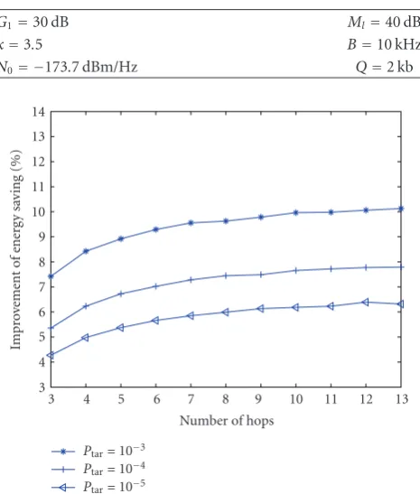
Table1: System parameters.
G1=30 dB Ml=40 dB
κ=3.5 B=10 kHz
N0= −173.7 dBm/Hz Q=2 kb
13 12 11 10 9 8 7 6 5 4 3
Number of hops Ptar=10−3
Ptar=10−4 Ptar=10−5 3
4 5 6 7 8 9 10 11 12 13 14
Im
pr
o
vement
o
f
energ
y
sa
ving
(%)
Figure 1: Average improved performance due to optimum BER allocations under different hop lengths for the loose delay case.
distribution, as this is shown in [8] to match very well the empirical hop length distribution when nodes are uniformly distributed across a finite square. The mean value of the hop length is set equal to 10 meters.
Figure 1 shows the simulation result regarding energy savings for differentPtar under different numbers of hops
in the loose delay case. For a given Ptar the performance
improvements are drawn as comparisons between optimally allocated BERs in all hops according tox∗ in (12), and the case when the per-hop BERs are evenly assigned as in [8], that is, byPbi=1− L
1−Ptar.Because of the random nature
of the route lengths, the gain for each route realization will be different; each dot drawn in Figure 1 is hence plotted after taking an average over 1000 randomly generated routes. Figure 1shows that by optimally allocating the BER along the route, the total energy consumption across the route could indeed be reduced compared to uniformly assigning BER, roughly by around 7% on the average.
One prominent feature we can see fromFigure 1is that the average energy gains clearly drop when Ptar decreases.
The reason for this could be seen from the objective function (5), where the BERs contribute to the energy budget by the terms ln(1/5xi), wherexirepresents the BER in each hop. The logarithm function is insensitive to changes in its argument when it is large. Therefore, when a lower target bit error rate is set up, the optimal BER assigned to each hop will accordingly become smaller. Hence, even if we optimally choose the BER, the performance gain will not be as obvious as in the largerPtarcase.
The second important feature from Figure 1 is that the performance gain grows larger as the number of hops increases. We may also explain this by means of the approximation ln(1−x)≈ −x, which holds wheneverx≈0. Sincexrepresents the BER, which is typically a very small value, we could then approximate the constraint (7) well as a linear equality constraint:
L
i=1
xi=Ptar. (14)
Now, we can use this constraint to compute λe instead of using (13). By recalculating the above steps and following exactly the same argument, this will give us the optimum solution xi∗ = Cdκi/λe, where the Lagrange multiplier λe could be obtained by satisfying the equality constraint in (14). This leads us to the approximate optimum solution
x∗=Ptar
dκ1
L
i=1diκ
,. . ., d κ L
L
i=1dκi
T
, y∗=[1,. . ., 1]T.
(15)
It can be seen from x∗ in (15) that for a given small
Ptar, the BER allocation scheme is only related to the hop
lengths in the route. We should also note that in (15), for one particular target route, the denominator Li=1dκ
i will become a constant. Therefore, the optimum BER allocation for a specific hopiis proportional to the current hop length
di powered by the path-loss exponentκ. This implies that we should allow larger error probabilities on those hops with long transmission distances, but that be very restrictive on the short hops. Thus, compared to the case where the per-hop BERs are evenly distributed, the energy savings are obtained by using relatively more power on the short hops, and relatively less on the long ones, as it costs much more transmit power to attain the same BER on a long hop than on a short hop. The result, compared tox∗in (12), directly and profoundly reveals the relation between the optimum results and the hop lengths, and it also matches our intuition.
This analytical result can also be used to understand the second feature mentioned above: why the energy saving gains become greater as the number of hops increases. This can be seen through a simple example, where we assume a route consisting only of two hops. Denote their lengths byd1and
d2, respectively, The total length of the route is set to be fixed,
that is,d1+d2=c. It is known from above that the optimum
BER allocations of this two-hop route is
Pb1=Ptar d
κ
1
d1κ+d2κ
, Pb2=Ptar d
κ
2
dκ1+dκ2
. (16)
We now explore the worst case where we have the max-imum total energy consumption. Equivalently, this means that we need to solve the following constrained optimization problem:
Maximize C·
dκ1ln
5Ptar d
κ
1
dκ
1+d2κ
+d2κln
5Ptar d
κ
2
dκ
1+dκ2
subject to d1+d2=c.
The functionxlogxis known to be strictly convex inx. Since the objective function is the sum of two such strictly convex functions with a sign reversal (Cis negative), it is a strictly concave function. It is not difficult to prove that this function reaches its maximum whend1=d2=c/2 which implies that
the power savings are minimum when the hop lengths are equally distributed, and any unevenly distributed hop lengths will result in a potential for further energy gain. In other words, the more the hop lengths deviate from the constant length, the more gain we can obtain.
As mentioned earlier, in the above simulations, we have assumed the hop lengths to be i.i.d. Rayleigh random variables. As the number of hops increases, we are then more likely to experience large deviations in the hop lengths across the route, which after optimization will result in a higher performance gain. However, Figure 1 also shows that all performance gain curves saturate as the hop number grows greater than 10. The reason is that, as the number of hops increases, though we generally deviate more from a uniform distribution of the hop length, at the same time there is also a larger probability of having a noticeable number of hops which will have approximately the same length, which actually contribute very little to the overall performance improvement. The relative gain is thus becoming more stable. In the next section, we will be able to quantify this effect more exactly, through a single parameter quantifying the maximum possible gain.
4. Tight Delay Constraint
4.1. Two Convex Subproblems. As previously emphasized,
if the delay constraint is inactive, then the time must be sufficiently large. The contrapositive of this implies thatif
the time is not sufficiently large, then the delay constraint must
be active.This means that the optimal solution will stay the
same if we rewrite the inequality constraint (9) as an equality, and it also means that we will have one more active constraint when writing the KKT equations. However, this will not help us further, since we still need to check the combinations of the rest of the inequality constraints. In this case, therefore numerical optimization algorithms must be used to search for the minimum. The change from inequality to equality does however facilitate the converging speed of the numerical algorithm (we used the MATLAB functionfminconto solve the optimization problem).
To aid the speed of the numerical optimization even more, further simplifications can also be explored, as will now be explained. If we assume thatyis given (i.e., we know the modulation order used in each hop), then the problem left will be the following optimization problem:
Minimize fx|y=C
For this model, sinceyis given, the objective function is a weighted sum of ln(1/5xi) over alli, which can easily be shown to be strictly convex with respect toxi forxi < 0.2. Constraint (19) is a strict inequality constraint; however, it is not hard to see that the function f(x |y) will be infinite and thus cannot reach its minimum at the pointxwhenever
xi =0 for i =1, 2,. . .,L. Therefore it is no harm for us to modify the constraint (19) to a constraint where equality is included, that is, xi ≥ 0, fori = 1, 2,. . .,L. Furthermore, we will again use the approximate linear equality constraint
L
i=1xi = Ptar, instead of the exact nonlinear constraint
(20). Hence, the optimization problem for a givenycan be rewritten as
It should be noted that the replacement of the nonlinear constraint by the linear constraint will not introduce much of a gap between the exact and approximate optimal gains. We can see this fromFigure 1where the order of magnitude of variation on the target BER only results in a few percentage changes in the gain. This suggests that BER allocations in general have limited impact in the energy savings, and we will show later that compared with the gain achieved by introducing optimal transmission rate allocations, this gap can be ignored.
The constraints we have now consist of several sets of linear inequality constraints, and one linear equality constraint. Since the linear functions are also convex, the constraints (22) and (23) together define a convex feasible domain. Hence, by the convex KKT theorem (see, e.g., [13]), any KKT point will also be the global minimum. The previously noted fact that the minimum cannot exist at any point with xi = 0, fori = 1, 2,. . .,L, implies that none of the constraints in (22) will be active at the minimum point, and thus they could be excluded when applying the KKT conditions. On the other hand, we know that the BER constraint (23) will surely be active; therefore, applying the KKT theorem gives us the following equation:
−C
By solving this equation, we get the following optimum solution for any giveny:
where λe satisfies the equality constraint
L
i=1xi∗ = Ptar.
Therefore, this gives us the following global minimum for problem (21):
One meaning of the above derived solution is that it tells how to find the optimum BERs along the route, given the transmission rate of all the nodes. Another is that it suggests that the existence of a set of mappings, denoted by
x1∗ = m1(y),x2∗ = m2(y),. . .,x∗L = mL(y), which together make sure thatx∗ is the global minimum for the function
f(x | y) defined above. We can thus eliminate xi in the problem formulation, and the problem is now reduced to finding they∗which can minimize the original problem (5). The whole problem under a tight delay constraint can now be written as the following optimization problem:
Minimize fy=C
Thus, we have reduced the number of unknowns by a factor of two, which will help to increase the numerical algorithm’s search speed. The first constraint above is a set of linear inequality constraints, which naturally define a convex set. The second constraint is in fact a set of nonlinear inequality constraints. Hence, if we definec(y)=L
i=1(1/ yi), all entries strictly positive. Hence, it is a positive definite matrix, which in turn implies thatc(y) is a strictly convex function. The argument that the level set of a convex function is also convex (see, e.g., [14, Chapter 1]) makes (29) define a convex set. Moreover, since (28) is a set of linear inequality constraints, the argument of the intersection of convex sets being convex guarantees that the problem is defined on a convex feasible domain.
It should be noted that, as we have argued above, (29) can be written as an equality. However, to prove the convexity, it is admissible if we extend the domain to include the inequality cases, since we are still in the feasible domain. Furthermore, given an initialyvalue, due to the mapping of
(26), the problem in (27)–(29) is equivalent to the following optimization problem:
This objective function can be proven to be convex with respect to y (see the appendix). It suggests that we can find a unique global minimum y that corresponds to the givenx, which is also uniquely determined by the previous ythrough (26). Hence, the search can operate in an iterative manner. From an initialy1we find an optimumx1∗through
(26), and this x∗ in turn updatey1 to a new value of y2
by solving problem (31). In particular, both subproblems are constrained convex optimization problems, which ensure that the extremum found is unique and global for each iteration. The above iterative process repeats until bothxand yconverge. In order to find the global minimum to the whole problem, different initial values ofy(which should comply with the constraints (32) and (33)) should be tested.
4.2. Numerical Results and Analysis. The system performance
under optimum configuration is depicted inFigure 2, where average energy savings are obtained by jointly optimizing the transmission rate and the BER allocation. In particular, the target BER is set toPtar = 10−3 for all curves. The gain is
plotted as a comparison between the optimal configuration and the case when both the BERs and transmission rates are evenly assigned along the route. To be consistent with simulation in the loose delay case, the hop length was still assumed to obey a Rayleigh distribution with mean value 10 meters. The curve is drawn over different values of the delay constraint. In particular, T = 1 implies the situation that if every node adopts BPSK, the delay constraint will be just met.
From the figure, all the curves indicate that we can have a significant average energy saving gain when the delay constraint is tight. For instance, in the 11 hops case, when the delay constraint is 0.1 (i.e., the acceptable delay is only 10% of what we would have when BPSK is used) the gain could be as much as 63%. Even in the 3 hops case, the gain could be close to 50%. This suggests that it is crucial to use adaptive transmissions if the delay requirement is tight and an energy efficient solution is required.
0.9 0.8 0.7 0.6 0.5 0.4 0.3 0.2 0.1
Delay constraintT 3 hops
8 hops
11 hops 13 hops 0
10 20 30 40 50 60 70
Energ
y
sa
ving
gains
(%)
Figure2: Energy savings for different number of hops under a tight
delay constraint with target BER=10−3.
gradually converge to BPSK. Thus the system’s performance will eventually approach the previously discussed loose delay case, in which only the per-hop BERs and corresponding transmit powers are optimally allocated.
Attention should also be paid to the gain performance as the hop number increases. It first improves fast over the whole range of delays; then, however, very little performance gain is obtained by going from 11 hops to 13 hops. This suggests that there is a performance limit; that is, the gain converges to a constant value as the number of hops grows very large. This phenomenon can be connected with the loose delay case where the BERs were optimally allocated. In Figure 1we also observed that the improvement slows down when the number of hops grows very large. This implies that the system’s maximum gain is limited by some inherent factor, to be explained next.
4.3. The D Parameter and Its Impact. It is important to
understand the reason why substantial energy savings can be acquired when the number of hops goes from 3 to 8 in Figure 2. In the loose delay case, we demonstrated that the gain comes from the uneven distribution of the hop lengths. Similarly, if all hops had the same length, then the best strategy would be to let all hops use the same transmission rate and be assigned the same BER, which would produce no gain at all.
Also in the tight delay case, the gain actually comes from the differences in the hop lengths. These differences are ultimately controlled by the degree of deviation from the uniform hop length distribution. To characterize this effect, we hereby define thisdegree of deviation,D, by the ratio of the variance to the square of the mean:
D=E
d2−E2[d]
E2[d] =
Ed2
E2[d]−1. (34)
Specifically, theDparameter for the Rayleigh distribution is in fact a constant, (4−π)/π ≈0.273. This explains why the simulation above indicates a performance limit, since as the hop number increases, the degree of deviation experienced in the hop length distribution of one route realization will statistically converge to this value. In the case shown in Figure 2, 11 hops are actually already large enough for this statistical convergence to occur, hence there is very limited gain by going from 11 hops to 13 hops. With a smaller number of hops, this situation of deviation effect is relatively less evident, which explains why the gain increment is more obvious for fewer hops.
The above analysis, on the other hand, also suggests that a higher performance gain could be obtained if theD
parameter grows large. To verify this, we assume that the distancedobeys a Gamma distribution instead of Rayleigh and carry out a new simulation under this assumption. The probability density function of the Gamma distribution is defined by two parameterskandθand is given by
f(d;k,θ)=dk−1 e−d/θ
θkΓ(k), ford >0, k,θ >0, (35)
where Γ denotes the gamma function. The mean value is
kθ, and the variance iskθ2. Therefore, theDparameter for
Gamma distribution isD = 1/k.To be consistent with the simulation carried out previously, again we set the mean distance to be 10 meters, but with several differentkandθ
values such that theDparameter is varying. ThePtaris set
to be 10−3, and we choose a route consisting of 11 hops with
delay set to be 0.3.
Figure 3shows the results. We see a clear improvement when increasing the D parameter. It should be noted that the energy gain depicted in this figure is an average, since the hop lengths in a route are random variables. Figure 3 should thus be treated as an indicator of the average possible energy gain on the network level, since in an ad hoc network, communication can take place between arbitrary nodes, and hop lengths in the routes given by the routing algorithm can be random. It should also be noted that, in reality, if one particular route is given, it is more proper to configure the route according to the situation, since we might encounter the case where the network as a whole has a small overall
Dvalue, but a specific route inside might have a large hop length deviation, implying that a large energy saving gain can be achieved. Therefore, it is crucial to measure theD
parameter of a specific route of interest.
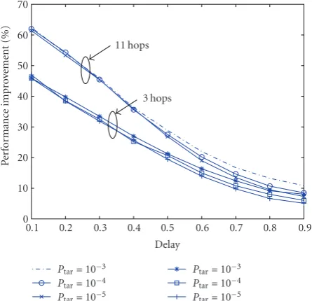
Another thing we have not investigated so far is how the target BERPtar affects the system performance in the tight
delay constraint case. As we saw in the above analysis, for a Rayleigh hop length distribution, the system approaches a limit after approximately 11 hops. Therefore, we choose two representative numbers of hops, 3 and 11 hops, and run the simulations under differentPtarvalues.
0.9 0.8 0.7 0.6 0.5 0.4 0.3 0.2 0.1
Dparameter 20
25 30 35 40 45 50 55 60 65 70
Energ
y
sa
ving
gains
(%)
Figure 3: Performance improvement for different Dparameters under a 11 hops route with delay constraintT = 0.3 and target BER=10−3.
0.9 0.8 0.7 0.6 0.5 0.4 0.3 0.2 0.1
Delay Ptar=10−3
Ptar=10−4 Ptar=10−5
Ptar=10−3 Ptar=10−4 Ptar=10−5 0
10 20 30 40 50 60 70
P
erfor
manc
e
impr
o
ve
ment
(%) 11 hops
3 hops
Figure4: Performance improvement for different delay constraints
under differentPtar.
general, the average performance is nearly the same as in Figure 2. Within each hop number, the curves are very close to each other, which means that there is no significant difference in relative energy saving gains on the average as we varyPtar. We also notice that as the delay become larger, the
discrepancies of the curves within the same cluster become more apparent. This is because, when the delay constraint is tight, the optimal BER assignment does not affect the average performance significantly, since at this point, the modulation order is very high. Thus the energy consumed by the modulation is dominant; whereas when the delay requirement is sufficiently loose, the modulation order will drop, and the energy spent on BER adaptation starts to come into play.
5. Circuit Power Consumption and
Peak Power Constraints
When the communication distance is short, it has been shown that the circuit power consumption is approximately on the same order of magnitude as the transmission power and should be taken into account in the system optimization [11]. To keep this work fit for general ad hoc networks where transmission energy is most often dominant, circuit power consideration was however not particularly addressed so far. Also, the circuit power consumption, including the power of filters and power amplifiers, will be dependent on the practical parameters in use, such as bandwidth and PA efficiency. The power consumption in the circuitry can however be modeled as a given constant for one specific transceiver pair during the transmission. If we denote this constant byPcir, the energy dissipated on the circuit along
the whole route can be written as
PcirQ
B
L
i=1
1
yi, foryi≥1. (36)
Equation (36) is a function ofyand it is of similar form as (29), which was proven to be convex. Hence, taking circuit power consumption into account preserves the convexity.
Similar to circuitry power consumption, peak power constraints have not been addressed either. One reason was that this would depend very much on specific implementa-tion details such as the type of battery installed, the power shared by the other components other than the transceiver such as the sensing unit, and the central processing unit. Another reason was that the peak power constraint might be different from node to node in a particular route, since nodes may have different residual energy. However, we can show that adding a peak power constraint also preserves the convexity. If we denote the maximum available transmission power on nodeiasPni, then this peak power constraint on nodeican be formulated as
1
7(N0B) ln
1
xi
21.9yi+ 1≤P
ni, foryi≥1. (37)
It can be seen that the constraint above defines a convex set if xi is given. Similarly,xi is linked to yi through (26). Therefore, for each iteration under an given initial value of y, the problem in (27) remains convex. Moreover, it is foreseeable that the circuit power consumption and the peak power constraint only function as setting up an upper and lower bound for the feasiblex,y, and neither of them will lead to a fundamental change of the results we get so far.
6. Conclusions
seen that by using the KKT theorem, the delay constraint divides the problem into two cases: the loose delay and tight delay case. In the loose delay case, an analytical solution was obtained, and the problem was proved to be equivalent to the question of how to optimally assign BERs along the route. Under a pure path-loss channel model, we have also shown that the optimal BER allocation scheme for a given target bit error rate, perhaps somewhat surprisingly, is only related to the hop lengthsdi.
In the tight delay case a numerical optimization algo-rithm has to be employed to solve the problem. We could however reduce the dimensions of the original problem by a factor of 2 through a unique mapping, which enabled the search algorithm to operate in an iterative manner. Simulations showed that large energy savings are possible, especially when the delay constraint is tight. At the same time, we also noticed that the energy saving performance seems to converge to a certain limit as the number of hops increases. A parameter D
measuring this limit was defined accordingly. Simulation results substantiate the validity of the parameter definition by indicating that more energy saving gain is possible asD
increases.
It should be noted that, to keep the problem’s generality, the problem has been analyzed on the basis of the most general physical layer QoS constraints, that is, the packet quality constraint (in terms of BER) and the delay constraint. Peak power constraints and circuit power consumption were not addressed, as these two parameters are highly dependent on the specific hardware implementations. However, we can show that these two constraints will not alter the convexity of the feasible domain, which implies that adding these two constraints would not fundamentally influence the analysis in the paper. Adding these two constraints can be thought of as imposing two additional bounds on the domain ofx andy, again indicating that they will not change the results fundamentally.
It should also be noted that in this paper, the trans-mission rate at each hop is assumed to be a continuous variable. However, in practical implementations, a discretiza-tion operadiscretiza-tion is needed since only integer number of constellation size can be supported. How to optimally do the discretization and to analyze in detail the performance after discretization are beyond the scope of this paper and is a topic for further research. Work on discrete rates to achieve the maximum average spectral efficiency can be found in [15]. In addition, analysis based on other modulation schemes other than MPSK is definitely worthy of studying. This can be useful for example in well-powered ad hoc networks such as in multimedia WSNs, where spectral efficiency is more emphasized. In addition, due to the dense traffic properties in such cases, packet collisions and queuing delay should also be taken into account.
Finally, our proposed work can also be combined with routing protocol design. Specifically, it can be added as a measure for the route decision mechanism and help to identify the least energy-consuming route among several options after route configuration.
Appendix
The Function
q
and Its Properties
The functionqis defined as
q(x)=21.9x+ 11
x. (A.1)
Now we prove that the functionq(x) is a positive, monoton-ically increasing convex function forx ≥1. The first-order derivative ofq(x) is
q(x)= [(1.9 ln 2)x−1]21.9x−1
x2 . (A.2)
It is easy to verify that q(x) is greater than 0 for x ≥ 1. Meanwhile,q(1)≈2.732>0. Henceq(x) is strictly positive and monotonically increasing. The second-order derivative ofq(x) is
q(x)= (1.9 ln 2)
221.9xx3−(1.9 ln 2·x−1)21.9x−12x
x4
(A.3)
>
(1.9 ln 2)2x2−2(1.9 ln 2)x+ 1 x21.9x
x4 . (A.4)
The term [(1.9 ln 2)2x2−2(1.9 ln 2)x+1] in (A.4) is a
second-order polynomial, which is increasing and strictly positive for
x ≥ 1. The linear functionxand the exponential function 21.9xare both increasing and positive forx≥1. Henceq(x) is strictly positive when x ≥ 1. We conclude that q(x) is strictly convex forx ≥ 1. Therefore,q(x) is monotonically increasing and convex forx≥1.
Acknowledgments
This work was carried out and supported by the NORDITE/NFR(VERDIKT) project CROPS. The authors are grateful to Dr. Anna Kim for helpful discussions.
References
[1] G. Karlsson, S. Lindfors, M. Skoglund, and G.∅ien, “Cross-layer optimization in short-range wireless sensor networks (CROPS),” Technical Part, http://www.ee.kth.se/commth/ projects/CROPS/docs/.
[2] A. J. Goldsmith and S. B. Wicker, “Design challenges for energy-constrained ad hoc wireless networks,”IEEE Wireless Communications, vol. 9, no. 4, pp. 8–27, 2002.
[3] V. Raghunathan, C. Schurgers, S. Park, and M. B. Srivastava, “Energy-aware wireless microsensor networks,” IEEE Signal Processing Magazine, vol. 19, no. 2, pp. 40–50, 2002.
[4] M. Younis, M. Youssef, and K. Arisha, “Energy-aware routing in cluster-based sensor networks,” inProceedings of the 10th IEEE/ACM International Symposium on Modeling, Analysis and Simulation of Computer and Telecommunication Systems (MASCOTS ’02), Fort Worth, Tex, USA, October 2002. [5] R. Shah and J. Rabaey, “Energy aware routing for low energy
[6] S. D. Muruganathan, D. C. F. Ma, R. I. Bhasin, and A. O. Fapojuwo, “A centralized energy-efficient routing protocol for wireless sensor networks,” IEEE Communications Magazine, vol. 43, no. 3, pp. S8–S13, 2005.
[7] L. Yang, H.-C. Yang, and K. Wu, “Minimum-energy route configuration for wireless ad hoc networks,” in Proceedings of the 25th IEEE International Performance, Computing, and Communications Conference (IPCCC ’06), pp. 9–14, Phoenix, Ariz, USA, April 2006.
[8] E. Krogsveen, C. Wang, G. E.∅ien, and S. Lindfors, “Energy-efficient adaptive route configuration in short-range wireless ad-hoc networks,” inProceedings of the 4th IEEE Internatilonal Symposium on Wireless Communication Systems (ISWCS ’07), pp. 292–296, Trondheim, Norway, October 2007.
[9] C. M. Wang, L. G. Yin, and G. ∅ien, “Adaptive route configuration for increased energy efficiency in wireless sensor networks,” in Proceedings of the 5th International Confer-ence on Broadband Communications, Networks, and Systems (CONET ’08), pp. 16–23, London, UK, September 2008. [10] J. Nocedal and S. J. Wright,Numerical Optimization, Springer,
New York, NY, USA, 2nd edition, 2006.
[11] S. Cui, A. J. Goldsmith, and A. Bahai, “Energy-constrained modulation optimization,” IEEE Transactions on Wireless Communications, vol. 4, no. 5, pp. 2349–2360, 2005.
[12] J. N. Al-Karaki and A. E. Kamal, “Routing techniques in wire-less sensor networks: a survey,”IEEE Wireless Communications, vol. 11, no. 6, pp. 6–28, 2004.
[13] H. E. Krogstad, “The Karush-Kuhn-Tucker Theorem,”http:// www.math.ntnu.no/∼hek/Optimering2007/KKT2007ver21feb .pdf
[14] D. P. Bertsekas, A. Nedic, and A. E. Ozdaglar,Convex Analysis and Optimization, Athena Scientific, Cambridge, Mass, USA, 2003.